NCEP-NCAR

Paek, H. and H.-P. Huang (2012), A comparison of the interannual variability in atmospheric angular momentum and length-of-day using multiple reanalysis data sets, J. Geophys. Res., 117, D20102, doi:10.1029/2012JD018105. 

This study performs an intercomparison of the interannual variability of atmospheric angular momentum (AAM) in eight reanalysis datasets for the post-1979 era.  The AAM data are further cross validated with the independent observation of length-of-day (LOD). The intercomparison reveals a close agreement among almost all reanalysis datasets, except that the AAM computed from the 20^th Century Reanalysis (20CR) has a noticeably lower correlation with LOD and with the AAM from other datasets.  This reduced correlation is related to the absence of coherent low-frequency variability, notably the Quasi-biennial Oscillation, in the stratospheric zonal wind in 20CR.  If the upper-level zonal wind in 20CR is replaced by its counterpart from a different reanalysis dataset, a higher value of the correlation is restored.  The correlation between the AAM and the Nino3.4 index of tropical Pacific SST is also computed for the reanalysis datasets. In this case, a close agreement is found among all, including 20CR, datasets. This indicates that the upward influence of SST on the tropospheric circulation is well captured by the data assimilation system of 20CR, which only explicitly incorporated the surface observations.  This study demonstrates the overall close agreement in the interannual variability of AAM among the reanalysis datasets.  This finding also reinforces the view expressed in a recent work by the authors that the most significant discrepancies among the reanalysis datasets are in the long-term mean and long-term trend. Paek and Huang 2012

   The time series of ∆LOD (red curve, converted to an equivalent ∆AAM using Eq. (3)) and ∆AAM (blue curve) from different reanalysis datasets: (a) NCEP R-1, (b) NCEP R-2, (c) CFSR, (d) 20CR, (e) ERA-40, (f) ERA-Interim, (g) JRA-25, and (h) MERRA. The time series of ∆Nino3.4 from HadISST is imposed as the green curve in panel (h). The units for ∆AAM and ∆Nino3.4 are 10²⁵ kg m² s^-1 and 1 °C, respectively. The time series for ∆AAM in panel (e) is slightly shorter due to the shorter record of the ERA-40 dataset.

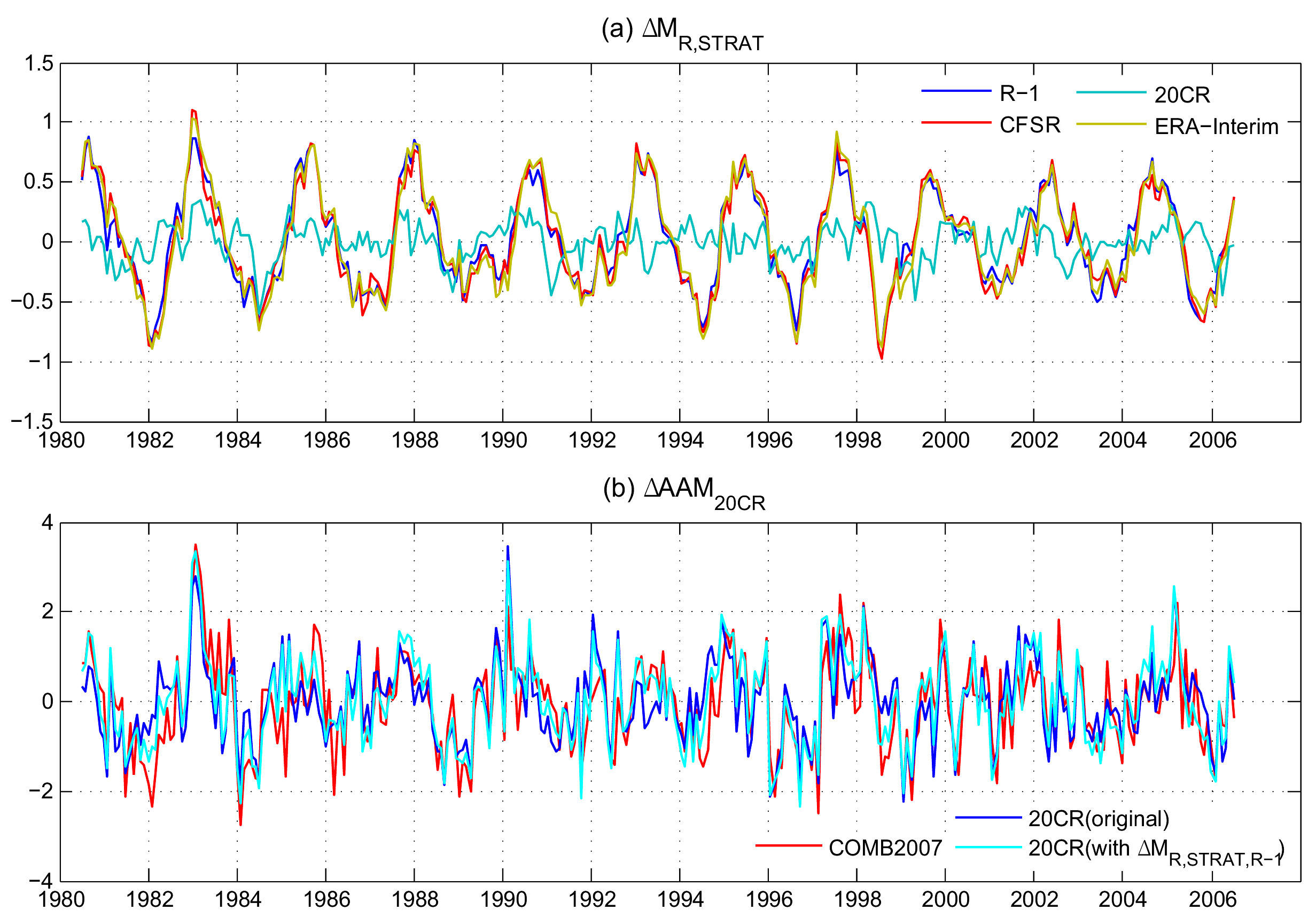
   The time series of ∆M_R,STRAT for four selected reanalysis datasets including 20CR. (b) The original (dark blue) and the modified ∆AAM (light blue) for 20CR. The modified ∆AAM is calculated by replacing the zonal wind in the stratosphere by that from NCEP R-1. See text for detail.  The time series of ∆LOD (converted to an equivalent ∆AAM) is also shown as the red curve. The unit for ∆AAM is 10²⁵ kg m² s^-1.

Zhang, Q., H. Körnich and K. Holmgren, 2012: How well do reanalyses represent the southern African precipitation? Clim. Dyn., DOI: 10.1007/s00382-012-1423-z.

http://dx.doi.org/10.1007/s00382-012-1423-z

Monthly-mean precipitation observations over southern Africa are used to evaluate the performance of eight global reanalyses: ERA-40, ERA-interim, JRA-25, MERRA, CFSR, NCEP-R1, NCEP-R2 and 20CRv2. All eight reanalyses reproduce the regionally averaged seasonal cycle fairly well; a few spatial mismatches with the observations are found in the climate mean for the rainy season. Principal component analyses show a dipole in the leading modes of all reanalyses, however with crucial differences in its spatial position.

Possible reasons for the differences between the reanalyses are discussed on the basis of the ERA-interim and 20CRv2 results. A comparison between the moisture transports shows that ERA-interim manifests a very strong moisture convergence over the eastern equatorial Atlantic, resulting in the strong precipitation here. This excessive convergence may be due to the water–vapor assimilation and convection parameterization. Over the Indian Ocean, the ITCZ is shifted northward in ERA-interim compared to its position in 20CRv2. This discrepancy is most likely attributable to the meridional SST gradients in the Indian Ocean which are significantly larger in the ERA-interim than those in the 20CRv2, and the resulting atmospheric response prevents a southward shift of the ITCZ.

Overall, the consistent description of the dynamical circulation of the atmosphere and the hydrological cycle appears as a crucial benchmark for reanalysis data. Based on our evaluation, the preferential reanalysis for investigating the climate variability over southern Africa is 20CRv2 that furthermore spans the longest time period, hence permitting the most precise investigations of interannual to decadal variability.

 

An intercomparison of the global relative angular momentum M_R in five reanalysis datasets, including the Twentieth Century Reanalysis (20CR), is performed for the second half of the twentieth century. The intercomparison forms a stringent test for 20CR because the variability of M_R is known to be strongly influenced by the variability of upper-tropospheric zonal wind whereas 20CR assimilated only surface observations. The analysis reveals good agreement for decadal-to-multidecadal variability among all of the datasets, including 20CR, for the second half of the twentieth century. The discrepancies among different datasets are mainly in the slowest component, the long-term trend, of M_R. Once the data are detrended, the resulting decadal-to-multidecadal variability shows even better agreement among all of the datasets. This result indicates that 20CR can be reliably used for the analysis of decadal-to-interdecadal variability in the pre-1950 era, provided that the data are properly detrended. As a quick application, it is found that the increase in M_Rduring the 1976/77 climate-shift event remains the sharpest over the entire period from 1871 to 2008 covered by 20CR. The nontrivial difference in the long-term trend between 20CR and the other reanalysis datasets found in this study provides a caution against using 20CR to determine the trend on the centennial time scale that is relevant to climate change. These conclusions are restricted to the quantities that depend strongly on the upper-tropospheric zonal wind, but the approach adopted in this work will be useful for future intercomparisons of the low-frequency behavior of other climate indices in the reanalysis datasets. Paek and Huang 2012.

   (a) The 5-year running averaged monthly anomalies of global relative angular momentum, ΔM_R, for the 5 reanalysis datasets. (b) Same as (a) but for ΔM₂₀₀, the angular momentum (per unit pressure thickness) calculated at only 200 hPa level.

   (a) The least-square quadratic fit (dashed curve) to ΔM_R for NCEP Reanalysis I, ERA-40, and 20CR for 1949-1978. (b) the “detrended” time series for the same period, with the quadratic curve removed from the time series. (c) Same as (a) but for 1979-2008 and with the addition of NCEP Reanalysis II and ERA-Interim.  (d) Same as (b) but for 1979-2008 and with the addition of NCEP Reanalysis II and ERA-Interim.

  (a) The global relative angular momentum, M_R, with the long-term mean retained, for the five reanalysis datasets. (b) Same as (a) but for M₂₀₀.  (c) Same as (a) but with the integration carried out only from 150-10hPa and 10°S-10°N to show the contribution from tropical upper atmosphere.

  (a) The summer (JJA)  climatology of zonal mean zonal wind from 1979-2008 for 20CR. (b) Same as (a) but for ERA-Interim. (c) The difference between 20CR and ERA-Interim, i.e., (b) minus (a). (d) is similar to (c) but for the difference between NCEP Reanalysis II and ERA-Interim.  (e)-(h) are similar to (a)-(d) but for winter (DJF). (i)-(l) are similar to (a)-(d) but for the annual mean.  (m) and (n) are the 1979-2008 linear trends for 20CR and ERA-Interim.  Contour intervals are 4 m s^-1 for (a), (b), (e), (f), (i), and (j);  1 m s^-1 for (c), (d), (g), (h), (k), (l), (m) and (n).

The extended intercomparison to CFSR and MERRA can be found at http://icr4.org/posters/Paek_AT-43.pdf.

Xue, Y., B. Huang, Z.-Z. Hu, A. Kumar, C. Wen, D. Behringer, and S. Nadiga, 2011: An assessment of oceanic variability in the NCEP Climate Forecast System Reanalysis. Clim. Dyn., 37 (11-12), 2511-2539, DOI: 10.1007/s00382-010-0954-4.

http://www.springerlink.com/content/x01q261216071647/

At the National Centers for Environmental Prediction (NCEP), a reanalysis of the atmosphere, ocean, sea ice and land over the period 1979-2009, referred to as the Climate Forecast System Reanalysis (CFSR), was recently completed. The oceanic component of CFSR includes many advances: (a) the MOM4 ocean model with an interactive sea-ice, (b) the 6 hour coupled model forecast as the first guess, (c) inclusion of the mean climatological river runoff, and (d) high spatial (0.5^o x 0.5^o) and temporal (hourly) model outputs. Since the CFSR will be used by many in initializing/validating ocean models and climate research, the primary motivation of the paper is to inform the user community about the saline features in the CFSR ocean component, and how the ocean reanalysis compares with in situ observations and previous reanalysis. The net ocean surface heat flux of the CFSR has smaller biases compared to the sum of the latent and sensible heat fluxes from the Objectively Analyzed air-sea Fluxes (OAFlux) and the shortwave and longwave radiation fluxes from the International Satellite Cloud Climatology Project (ISCCP-FD) than the NCEP/NCAR reanalysis (R1) and NCEP/DOE reanalysis (R2) in both the tropics and extratropics. The ocean surface wind stress of the CFSR has smaller biases and higher correlation with the ERA40 produced by the European Centre for Medium-Range Weather Forecasts than the R1 and R2, particularly in the tropical Indian and Pacific Ocean. The CFSR also has smaller errors compared to the QuickSCAT climatology for September 1999 to October 2009 than the R1 and R2. However, the trade winds of the CFSR in the central equatorial Pacific are too strong prior to 1999, and become close to observations once the ATOVS radiance data are assimilated in late 1998. A sudden reduction of easterly wind bias is related to the sudden onset of a warm bias in the eastern equatorial Pacific temperature around 1998/99. The sea surface height and top 300 meter heat content (HC300) of the CFSR compare with observations better than the GODAS in the tropical Indian Ocean and extratropics, but much worse in the tropical Atlantic, probably due to discontinuity in the deep ocean temperature and salinity caused by the six data streams of the CFSR. In terms of climate variability, the CFSR provides a good simulation of Tropical Instability Waves (TIW) and oceanic Kelvin waves in the tropical Pacific, and the dominant modes of HC300 that are associated with El Nino and Southern Oscillation, Indian Ocean Dipole, Pacific Decadal Oscillation and Atlantic Meridional Overturning Circulation.

Kumar, A., and Z.-Z. Hu, 2012: Uncertainty in the ocean-atmosphere feedbacks associated with ENSO in the reanalysis products. Clim. Dyn., 39 (3-4), 575-588. DOI: 10.1007/s00382-011-1104-3.



http://www.springerlink.com/content/w66j8vh1n826n711/



 

The evolution of El Niño-Southern Oscillation (ENSO) variability can be characterized by various ocean-atmosphere feedbacks, for example, the influence of ENSO related sea surface temperature (SST) variability on the low-level wind and surface heat fluxes in the equatorial tropical Pacific, which in turn affects the evolution of the SST.  An analysis of these feedbacks requires physically consistent observational data sets.  Availability of various reanalysis data sets produced during the last 15 years provides such an opportunity. A consolidated estimate of ocean surface fluxes based on multiple reanalyses also helps understand biases in ENSO predictions and simulations from climate models. 

In this paper, the intensity and the spatial structure of ocean-atmosphere feedback terms (precipitation, surface wind stress, and ocean surface heat flux) associated with ENSO are evaluated for six different reanalysis products.  The analysis provides an estimate for the feedback terms that could be used for model validation studies.  The analysis includes the robustness of the estimate across different reanalyses. Results show that one of the “coupled” reanalysis among the six investigated is closer to the ensemble mean of the results, suggesting that the coupled data assimilation may have the potential to better capture the overall atmosphere-ocean feedback processes associated with ENSO than the uncoupled ones.

Many white papers, published papers, and other reports have been issued relating to reanalyses, their current status, and recommendations for improvements.  Please include such reports below in reverse chronological order, with links to a Discussion reanalyses.org page which summarizes the report and a link to the Full Report itself. 

Fujiwara, M., J. S. Wright, G. L. Manney, L. J. Gray, J. Anstey, T. Birner, S. Davis, E. P. Gerber, V. L. Harvey, M. I. Hegglin, C. R. Homeyer, J. A. Knox, K. Krüger, A. Lambert, C. S. Long, P. Martineau, A. Molod, B. M. Monge-Sanz, M. L. Santee, S. Tegtmeier, S. Chabrillat, D. G. H. Tan, D. R. Jackson, S. Polavarapu, G. P. Compo, R. Dragani, W. Ebisuzaki, Y. Harada, C. Kobayashi, W. McCarty, K. Onogi, S. Pawson, A. Simmons, K. Wargan, J. S. Whitaker, and C.-Z. Zou: Introduction to the SPARC Reanalysis Intercomparison Project (S-RIP) and overview of the reanalysis systems, Atmos. Chem. Phys., 17, 1417-1452, doi:10.5194/acp-17-1417-2017, 2017. Link to Paper. 

Compo, G., J. Carton, X. Dong, A. Kumar, S. Saha, J. S. Woollen, L. Yu, and H. M. Archambault, 2016: Report from the NOAA Climate Reanalysis Task Force Technical Workshop. NOAA Technical Report OAR CPO-4, Silver Spring, MD. doi: 10.7289/V53J39ZZ. Full Report.

Bosilovich, M.G, J.-N.Thépaut, O. Kazutoshi, A. Kumar, D. Dee and Otis Brown, 2015: WCRP Task Team for Intercomparison of ReAnalyses (TIRA). White Paper. Full Report.

CORE CLIMAX, 2014: Procedure for comparing reanalyses, and comparing reanalyses to assimilated observations and CDRs. COordinating Earth observation data validation for RE-analysis for CLIMAte ServiceS, Grant agreement No: 313085, Deliverable D5.53, pp 45. Full report

Bosilovich, M. G., J. Kennedy, D. Dee, R. Allan and A. O’Neill, 2013: On the Reprocessing and Reanalysis of Observations for Climate, Climate Science for Serving Society: Research, Modelling and Prediction Priorities. G. R. Asrar and J. W. Hurrell, Eds. Springer, in press. Full Report. Discussion Page. 

Bosilovich, M.G., M. Rixen, P. van Oevelen, G. Asrar, G. Compo, K. Onogi, A. Simmons, K. Trenberth, D. Behringer, T. H. Bhuiyan, S. Capps, A. Chaudhuri, J. Chen, L. Chen, N. Colasacco-Thumm, M. G. Escobar, C.R. Ferguson, T. Ishibashi, M.L.R. Liberato, J. Meng, A. Molod, P. Poli, J. Roundy, K. Willett, J. Woollen,R. Yang, 2012: Report of the 4th World Climate Research Programme International Conference on Reanalyses, Silver Spring, Maryland, USA, 7-11 May 2012. WCRP Report 12/2012. Full Report. Discussion Page.

Rienecker, M.M., D. Dee, J. Woollen, G.P. Compo, K. Onogi, R. Gelaro, M.G. Bosilovich, A. da Silva, S. Pawson, S. Schubert, M. Suarez, D. Barker, H. Kamahori, R. Kistler, and S. Saha, 2012: Atmospheric Reanalyses—Recent Progress and Prospects for the Future. A Report from a Technical Workshop, April 2010. NASA Technical Report Series on Global Modeling and Data Assimilation, NASA TM–2012-104606, Vol. 29, 56 pp. Full Report. Discussion Page.

Climate Change Science Program, 2008: Weather and Climate Extremes in a Changing Climate. Regions of Focus: North America, Hawaii, Caribbean, and U.S. Pacific Islands. A Report by the U.S. Climate Change Science Program and the Subcommittee on Global Change Research. [Thomas R. Karl, Gerald A. Meehl, Christopher D. Miller, Susan J. Hassol, Anne M. Waple, and William L. Murray (eds.)]. Department of Commerce, NOAA's National Climatic Data Center, Washington, D.C., USA, 164 pp. Full Report.

Climate Change Science Program, 2008: Reanalysis of Historical Climate Data for Key Atmospheric Features: Implications for Attribution of Causes of Observed Change. A Report by the U.S. Climate Change Science Program and the Subcommittee on Global Change Research [Randall Dole, Martin Hoerling, and Siegfried Schubert (eds.)]. National Oceanic and Atmospheric Administration, National Climatic Data Center, Asheville, NC, 156 pp. Full Report.

Lermusiaux, P.F.J.,  P. Malanotte-Rizzoli, D. Stammer, J. Carton, J. Cummings, and A.M. Moore, 2006: Progress and Prospects in U.S. Data Assimilation in Ocean Research. Oceanography, 19, 172-183. Full Report.

Arkin, P., E. Kalnay, J. Laver, S. Schubert, and K. Trenberth, 2003: Ongoing analysis of the climate system: A workshop report. NASA, NOAA, and NSF, 48 pp.  Full Report.

A recent publication on different Arctic cloud climatologies intercomparison shows a wide spread among observations and reanalyses. Reanalyses generally are not in a close agreement with satellite and surface observations of cloudiness in the Arctic. Several reanalyses show the highest values of total cloud fraction over the central part of the Arctic Ocean but not over the Norwegian Sea and the Barents Sea as observations do. The maximum and minimum of total cloud fraction in the annual cycle are shifted by 1-2 months compared to observations.

December-January-February and June-July-August mean of TCF over the Arctic (north of 60◦N) from different data.

The annual cycle of TCF.

Normalized pattern statistics showing differences among different observational and reanalyses TCF spatial distribution (Taylor diagrams).

Alexander Chernokulsky and Igor I. Mokhov, “Climatology of Total Cloudiness in the Arctic: An Intercomparison of Observations and Reanalyses,” Advances in Meteorology, vol. 2012, Article ID 542093, 15 pages, 2012. doi:10.1155/2012/542093

A set of web-based reanalysis intercomparison tools (WRIT) is available from the NOAA Physical Sciences Laboratory and University of Colorado CIRES.

WRIT Maps WRIT Time-series WRIT Correlations WRIT Trajectories WRIT Distributions

The "WRIT" Maps tool allows users to examine 20CR, ERA-Interim, ERA-20C, JRA-55, MERRA, MERRA-2, NCEP R1, NCEP R2, and NCEP CFSR reanalyses datasets. Pressure level data are available for most reanalyses, as well as 5 single level variables including sea level pressure, 2 m air temperature, 10 m winds, precipitation. Maps and pressure-level by longitude and pressure-level by latitude can be generated for monthly means, anomalies, and climatologies. Observational datasets have been made available that can be compared to 2m air temperature and precipitation. These quantities can be differenced between datasets.

Future enhancements include different time scales.

is also available from WRIT. It allows users to examine 20CR, ERA-Interim, ERA-20C, JRA-55, MERRA, MERRA-2, NCEP R1,  NCEP R2, and NCEP-CFSR as well as some observational dataset. Users can compare timeseries from different datasets, regions, variables and levels. Distributions, scatter plots, and auto-correlation are also available. Statistics for each timeseries including means, standaed deviations, slope and correlations are provided.

The "WRIT" Trajectory Tool is a new tool available from WRIT. It allows users to plot forward and backward trajectories from different reanalyses (currently NCEP R1, NCEP R2, and 20CR with more planned). Users can plot  the trajectories of one or more levels on a single plot. The output is plotted and is available as netCDF and as KMZ files suitable for Google Earth.

Other analysis products are planned.

Feedback and suggestions are welcome. Please give comments/issues/suggestions in the Post a comment or question below.

Acknowledgments

The Twentieth Century Reanalysis Project (20CR) used resources of the National Energy Research Scientific Computing Center managed by Lawrence Berkeley National Laboratory and of the Oak Ridge Leadership Computing Facility at Oak Ridge National Laboratory, which are supported by the Office of Science of the U.S. Department of Energy under Contract No. DE-AC02-05CH11231 and Contract No. DE-AC05-00OR22725, respectively. Support is provided by the U.S. Department of Energy, Office of Science Innovative and Novel Computational Impact on Theory and Experiment (DOE INCITE) program, and Office of Biological and Environmental Research (BER), and by the National Oceanic and Atmospheric Administration Climate Program Office. Data are freely available from NOAA, NCAR, the IRI, KNMI, and DOE NERSC.

NASA's Modern Era Retrospective analysis for Research and Applications (MERRA) was developed by the Global Modeling and Assimilation Office (GMAO) and produced through NASA's Modeling, Analysis and Prediction (MAP) program, and is freely available from the Goddard Earth Sciences (GES) Data Information Services center (DISC).

NCEP's Climate Forecast System Reanalysis (CFSR) was developed by the Environmental Modeling Center (EMC) and was partially funded through the NOAA Climate Program Office. It is available free to the public from both NCDC and NCAR.

The ERA-Interim reanalysis is being produced by the European Centre for Medium-Range Weather Forecasts (ECMWF) in Reading, UK. ERA-Interim data with near-real time updates are freely available from the ECMWF data server and from the CISL Data Archive at NCAR. 

WRIT contributes to the Atmospheric Circulation Reconstructions over the Earth (ACRE) Initiative.

WRIT is supported in part by NOAA and by the US Department of Energy Office of Science (BER).

Data Extraction

1. NCEI NOMADS and NCMP:  reanalysis (CFSR,NARR,R1,R2); NWP (NAM, GFS, RUC); GENS ensembles, SST
2. NOAA PSL Search and Plot. (R1,R2,20CR, NARR)
3. NOAA IRI (CFSR,20CR,R1,R2)
4. ECMWF: 
   1. ERA5: access via the Climate Data Store https://cds.climate.copernicus.eu/#!/home and https://cds-beta.climate.copernicus.eu/ 
   2. Alternative: https://www.ecmwf.int/en/forecasts/datasets/search 
5. NASA 
   1. MERRA: GES DISC Data Collections: MERRA
   2. MERRA-2: GES DISC Data Collections: MERRA-2
   3. MERRA and MERRA2 Data Subsetter  (variable list for MERRA-2)
6. NCAR, Highest-resolution files for all reanalyses, except MERRA. GRIB parameter field extraction using cURL, and some conversion to netCDF as noted. 
   1. JRA-25: Data Access > Web File Listing > Create Your Own File List (e.g. anl_p), use cURL or wget (for files).
   2. JRA-55
   3. ERA5, ERA-Interim
   4. CFSR - (also subset with net CDF format conversion)
   5. 20CR
   6. 20CRv2c
   7. 20CRv3
7. OpenDAP servers: 
   1. NOAA PSL (20CR,R1,R2,NARR), NCEP, MERRA2D, MERRA3D
   2. MERRA Gridded Innovations and Observations (GIO)
8. OpenGrADS.org: GrADS software with additional user functionality, including GUI for reanalyses including NCEP and MERRA
9. Earth System Grid Federation (CFSR, MERRA, 20CR, JRA-25, ERA-Interim) Obs4MIPS: Easy access to NetCDF reanalyses data of selected variables corresponding to the CMIP5 climate model output
10. GOAT: Geophysical Observations Analysis Tool for MATLAB

Step-by-Step Guide to obtaining data files

• Step by step descriptions of how to get the data at the reanalyses centers are available.

Post Processing Routines and Algorithms

1. Extrapolate MERRA pressure-level data below the surface

Webtools to plot/analyze data by Function

Basic Maps

1. NOAA IRI (CFSR,20CR,R1,R2)
2. NOAA PSL Search and Plot (20CR,R1,R2,NARR)
3. NASA MERRA: Uses Giovanni to produce maps or animations of some monthly fields. Can average over successive times.
4. NOAA NOMADS (CFSR,NARR,R1,R2)
5. ECMWF ERA-40, ERA-Interim (Plot maps)
6. NASA MERRA Atlas
7. NOAA/PSL Web-based Reanalysis Intercomparison Tool for maps makes user-selected reanalysis fields for monthly data. It can also difference two reanalyses or selected observational datasets with user-selected climatologies.
8. The Climate Reanalyzer makes user-selected reanalysis fields and differences for monthly data.
9. MeteoCentre provides pre-generated synoptic maps of SLP, 1000-500 thickness, and 500 hPa height (20CR and R1).
10. GOAT: Geophysical Observations Analysis Tool for MATLAB

Other Basic Geographic Plots

1. NOAA PSL:Crossections
2. NOAA PSL: Search and Plot
3. MERRA: Uses Giovanni to produce hovmollers of some monthly fields.
4. The Royal Netherlands Meteorological Institute (KNMI) Climate Explorer
5. GOAT: Management and Analysis of Geophysical-Data Made Simple for Matlab
6. Met Data Explorer

Hovmollers

1. NOAA/PSL: Hovmollers (R1)
2. IRI
3. GOAT: Geophysical Observations Analysis Tool:Management and Analysis of Geophysical-Data Made Simple for Matlab

Advanced Plots

1. NOAA PSL: Can plot monthly, daily and sub-daily of crossections from composite plotting pages (R1). Anomalies are available.
2. NOAA/PSL: Hovmollers of means, anomalies of daily data. Anomalies are available (R1).
3. GOAT: Temporal and spatial subsettting is supported via a GUI or built in function. Built-in calculation of anomalies and climatology. Superimpose or show the difference between two fields. Display land-cover or topography.

Composite Maps (Average different, possibly non-contiguous dates together)

1. NOAA PSL: Can plot composite maps and vertical crossectons from composite plotting pages on monthly, daily and sub-daily time scales for R1. Anomalies are available.
2. NOAA PSL: Can plot composite maps from plotting pages on monthly, daily and sub-daily timescales for 20CR. Anomalies are available. For monthly, plot composite maps of the 20CR ensemble spread (uncertainty).
3. GCOS/WGSP: Can plot composite maps of sea level pressure from plotting pages on monthly timescales. Anomalies are available.
4. WRIT maps: Can plot composite maps of a reanalysis or the difference of composites from two reanalyses.
5. GOAT: Can plot composites of non-contiguous dates.

Correlation Maps

1. NOAA PSL WRIT Correlations
2. NOAA PSL: From monthly NCEP/NCAR R1
3. KNMI
4. The Climate Reanalyzer (ERA-Interim, NCEP/NCAR R1, NCEP/DOE R2, 20CR, observational datasets: PRISM precipitation, ERSSTv3b)

Timeseries Plots

1. NOAA PSL Plot simple timeseries of NCEP/NCAR R1 and 20thC Reanalysis monthly variables
2. IRI Data Library
3. Met Data Explorer: Unidata
4. Web-based Reanalysis Intercomparison Tool for timeseries (WRIT) makes user-selected reanalysis timeseries, scatter plots, cross-correlation functions, and probability density functions for monthly data. It can also difference two reanalyses or selected observational datasets.
5. The Climate Reanalyzer makes user-selected reanalysis time series with land/ocean masking.

Timeseries Analysis

1. KNMI: Plot, compute annual cycle, filter and other tools available for time series analysis. Provides many climate/ocean time-series.
2. NOAA/PSL: Correlate and do some other simple analysis on pregenerated or user supplied monthly time-series
3. NOAA/PSL: Extract daily timeseries from datasets. Can supply user criteria (e.g. top 10 temperatures in January for a point). R1,20CR
4. NOAA/PSL: Extract monthly timeseries from datasets.  R1,20CR
5. IRI Data Library
6. NOAA PSL: Web-based Reanalysis Intercomparison Tool for timeseries (WRIT) makes user-selected reanalysis timeseries, scatter plots, cross-correlation functions, wavelets, and probability density functions for monthly data. It can also difference two reanalyses or selected observational datasets.

Google Earth

1. NOAA PSL: Create in KML plots (20CR, R1)

Miscellaneous

1. NOAA/PSL Lead/Lag for Composites
2. NOAA\/PSL Lead/Lag for Correlations (maps)
3. KNMI Smoothed fields, EOF, SVD and other analysis
4. NOAA/PSL WRIT Trajectory calculator (20CR, CFSR)

Applications that read/plot/analyze netCDF and/or grib data (non-web)

A complete list is at Unidata

1. NCL: NCAR Command Language (no longer updated but has full functionality)
2. GrADS: The Grid Analysis and Display System (GrADS)
3. IDV:  Integrated Data Viewer
4. Ferret: Data Visualization and Analysis: From NOAA/PMEL
5. NCO: NetCDF Operators. The NCO toolkit manipulates and analyzes data stored in netCDF-accessible formats, including DAP, HDF4, andHDF5. It exploits the geophysical expressivity of many CF (Climate & Forecast) metadata conventions, the flexible description of physical dimensions translated by UDUnits, the network transparency of OPeNDAP, the storage features (e.g., compression, chunking, groups) of HDF (the Hierarchical Data Format), and many powerful mathematical and statistical algorithms of GSL (the GNU Scientific Library). NCO is fast, powerful, and free.
6. CDO: Climate Data operators.  A collection of command-line operators to manipulate and analyze climate and numerical weather prediction data; includes support for netCDF-3, netCDF-4 and GRIB1, GRIB2, and other formats.
7. MATLAB
8. IDL: Interactive Data Language
9. CDAT Community Data Analysis Tools: CDAT: Note this will be replaced soon by xCDAT
10. xCDAT: xCDAT is an extension of xarray for climate data analysis on structured grids. It serves as a spiritual successor to the Community Data Analysis Tools (CDAT) library.
11. GOAT: Geophysical Observations Analysis Tool:  A MATLAB based tool that integrates with NetCDF files and OPeNDAP sources.

List of web-based tools for comparing reanalysis datasets:

 

• Web-based Reanalysis Intercomparison Tools

• KNMI Climate Explorer

• MERRA Atlas

• MERRA-2 Weather Maps

• JRA-55 Atlas

• The Climate Reanalyzer

• GOAT: Standardized dataset retrieval and analysis

GOAT (Geophysical Observation Analysis Tool) is a free MATLAB based tool for the analysis and visualization of various types of geophysical data.

GOAT archives all geophysical data in a consistent format thereby alleviating many of the annoyances related to the inconsistency of spatial and temporal resolutions, naming, units and file formats across the ever growing number of observed and simulated geophysical datasets.