Suggested Colors for Intercomparing Reanalysis Timeseries from S-RIP:

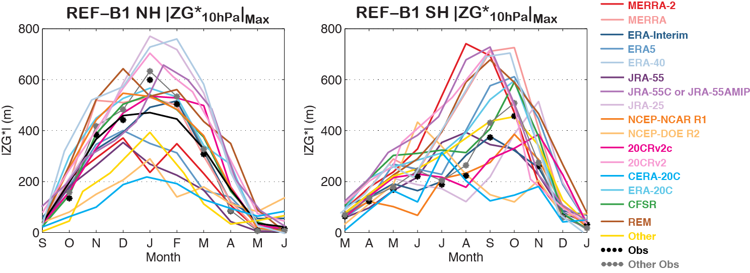
The Sparc Reanalysis Intercomparison Project (S-RIP --> https://s-rip.github.io/) has a suggested list of colors to use for comparing reanalysis time-series. The list can be viewed here https://s-rip.ees.hokudai.ac.jp/mediawiki/index.php/Notes_for_Authors --> https://s-rip.github.io/report/colourdefinition.html The colors are available in CVS format below, in NCL, and in XLS. The link to the S-RIP page has examples for Python and IDL --> https://s-rip.github.io/report/colourtables.html.

Note that the URLs have changed. 

The colors are available in CVS format below, in NCL, and in XLS. 

CSV:

r,g,b,c,m,y,k,RGB Hexadecimal,reanalysis

226, 31, 38,  0,86.28,83.19,11.37,  E21F26,  MERRA-2

246, 153, 153,  0,37.8,37.8,3.53,  F69999,  MERRA

41, 95, 138,  70.29,31.16,0,45.88,  295F8A,  ERA-Interim

95, 152, 198,  52.02,23.23,0,22.35,  5F98C6,  ERA5

175, 203, 227,  22.91,10.57,0,10.98,  AFCBE3,  ERA-40

114, 59, 122,  6.56,51.64,0,52.16,  723B7A,  JRA-55

173, 113, 181,  4.42,37.57,0,29.02,  AD71B5,  JRA-55C or JRA-55 AMIP

214, 184, 218,  1.83,15.6,0,14.51,  D6B8DA,  JRA-25

245, 126, 32,  0,48.57,86.94,3.92,  F57E20,  NCEP-R1

253, 191, 110,  0,24.51,56.52,0.78,  FDBF6E,  NCEP-R2

236, 0, 140,  0,100,40.68,7.45,  EC008C,  20CRv2c

247, 153, 209,  0,38.06,15.38,3.14,  F799D1,  20CRv2

0, 174, 239,  100,27.2,0,6.27,  00AEEF,  CERA-20C

96, 200, 232,  58.62,13.79,0,9.02,  60C8E8,  ERA-20C

52, 160, 72,  67.5,0,55,37.25,  34A048,  CFSR

179, 91, 40,  0,49.16,77.65,29.8,  B35B28,  REM

255,215,0,  0,15.69,100,0,  FFD700,  Other

0, 0, 0,  0,0,0,100,  000000,  Obs

119, 119, 119,  0,0,0,53.33,  777777,  Other Obs

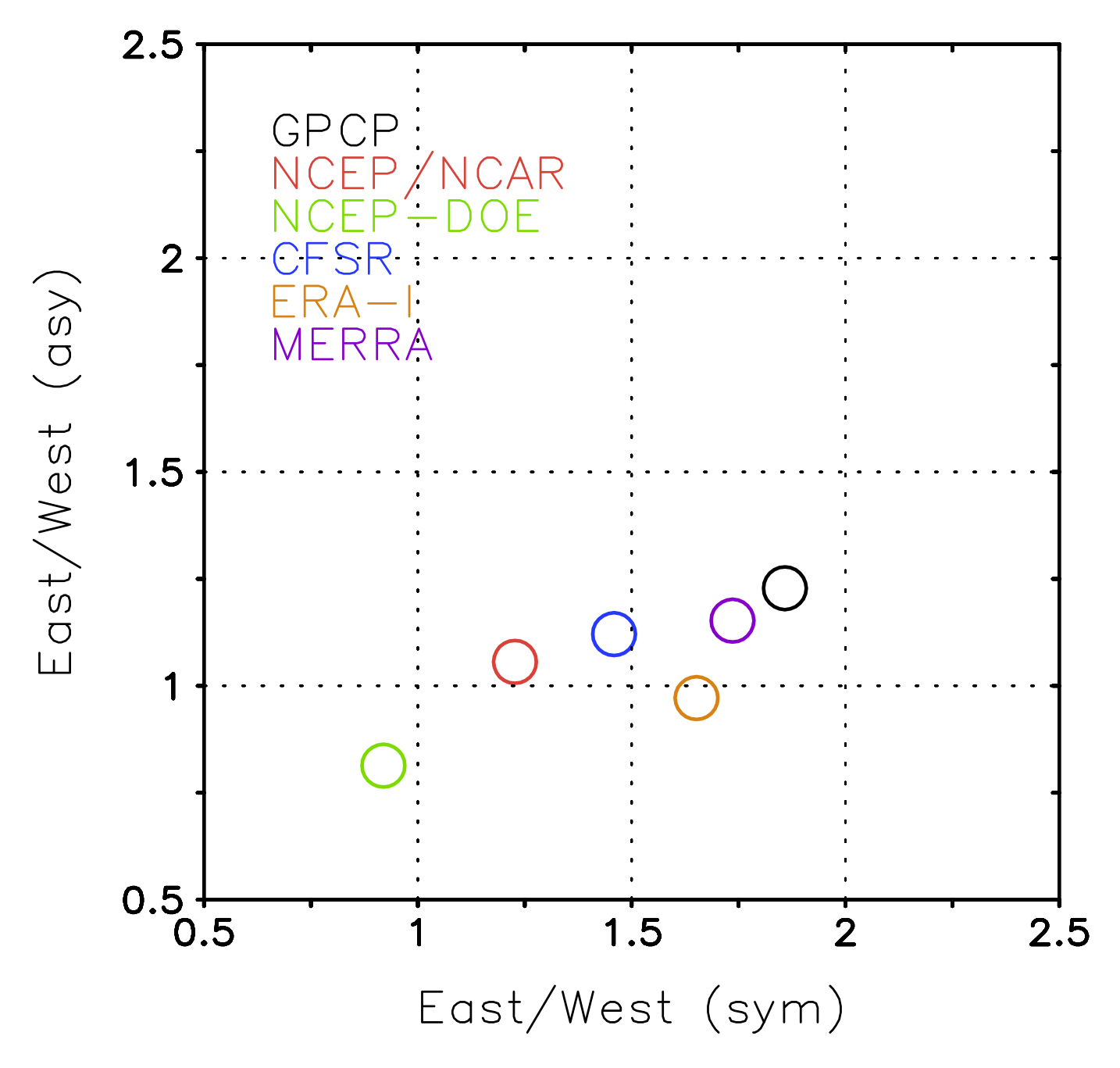
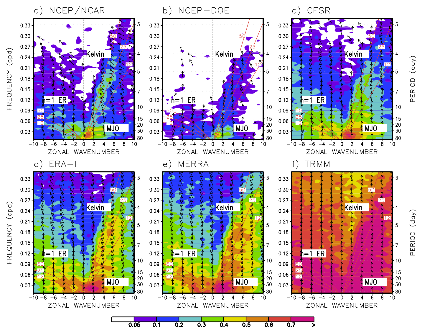
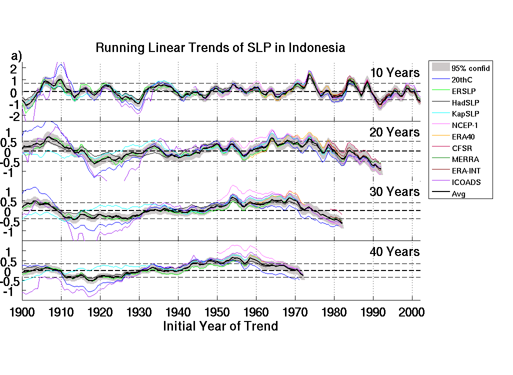
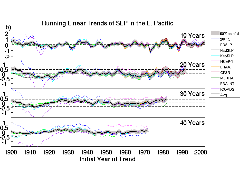
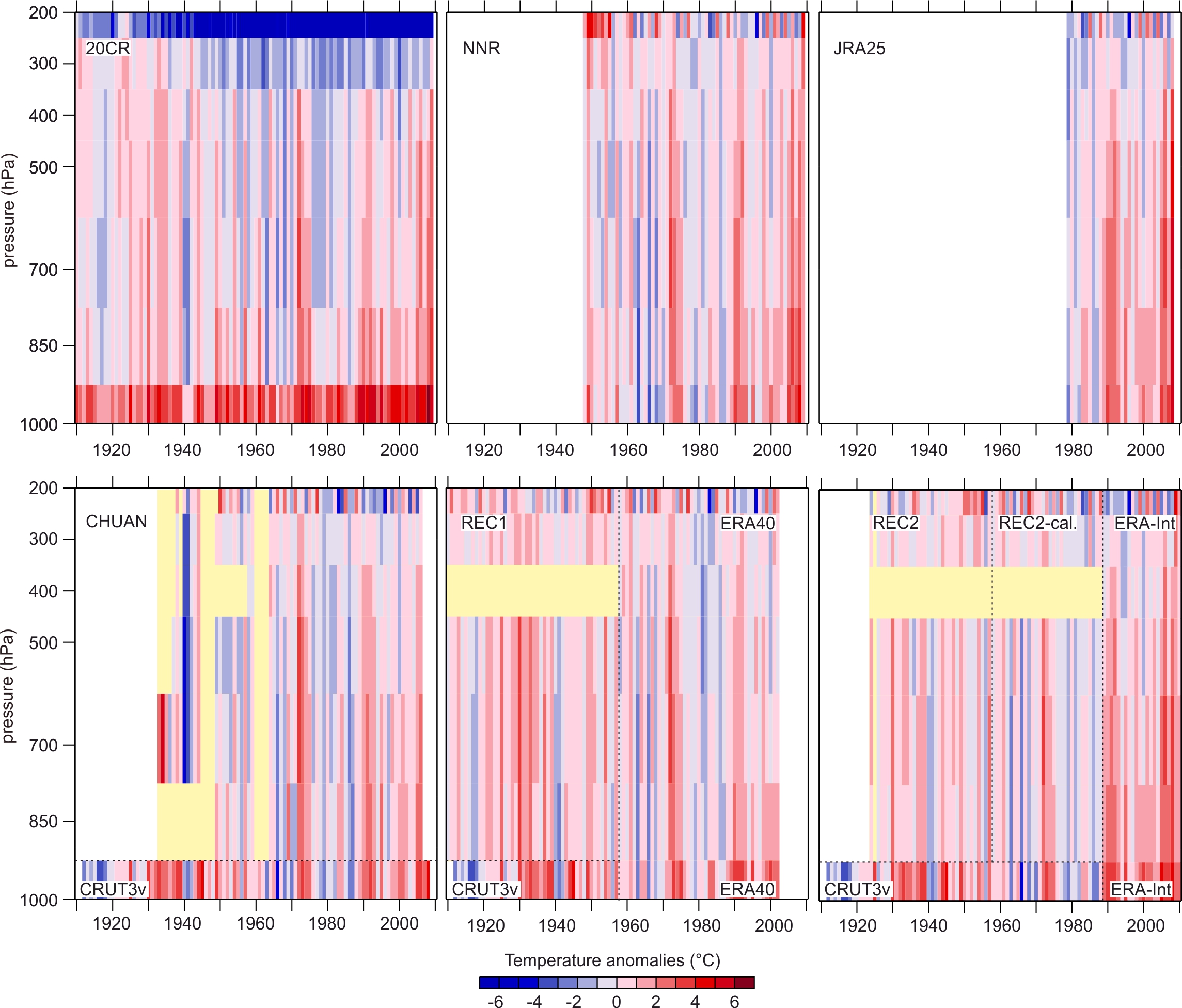
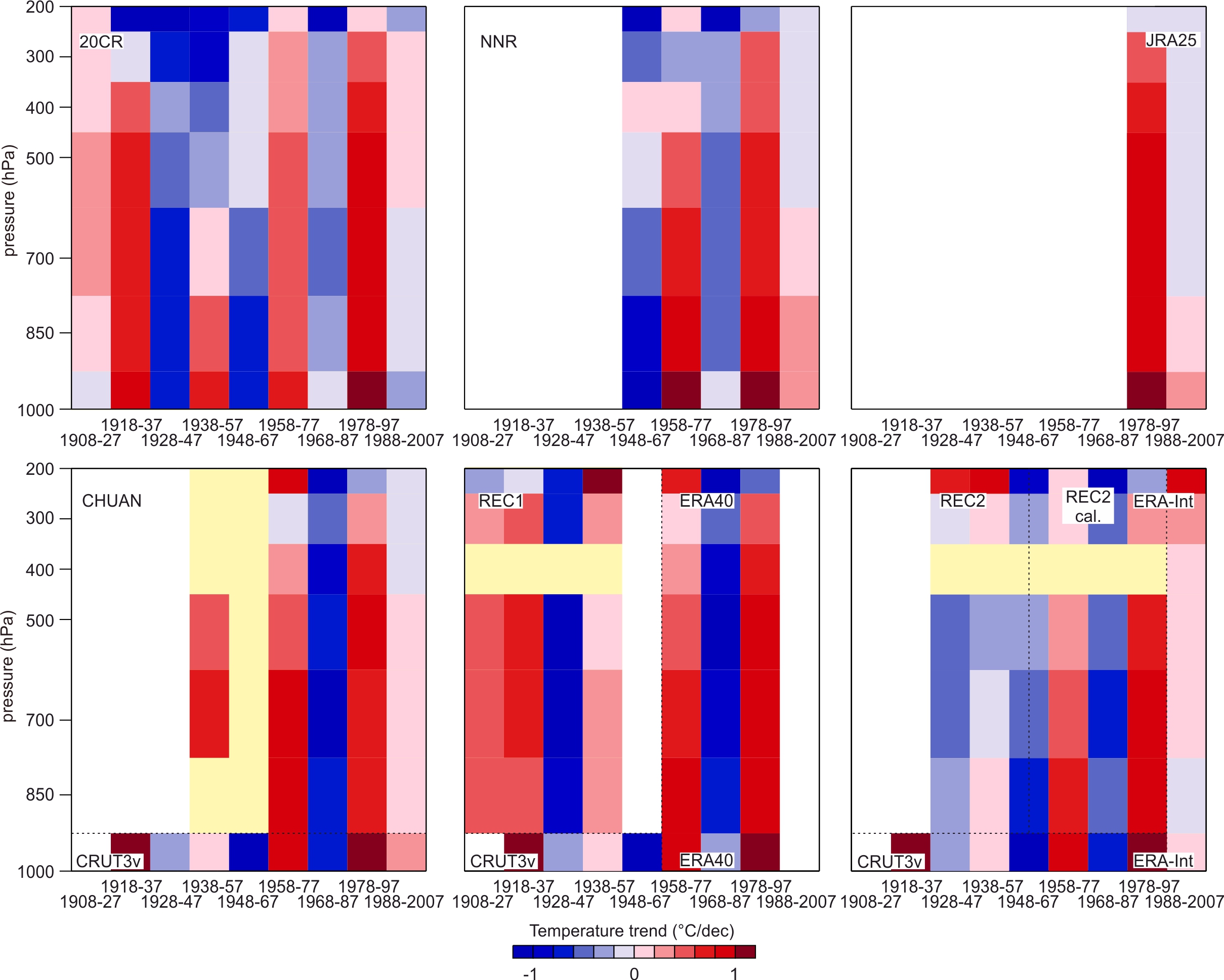
This image shows how the colors can be used.

Suggested Practices: Climatologies:

Use 1981-2010.

Land surface air temperature (SAT) is one of the most important variables in weather and climate studies, and its diurnal cycle and day-to-day variation are also needed for a variety of applications. Global long-term hourly SAT observational data, however, do not exist. While such hourly products could be obtained from global reanalyses, they are strongly affected by model parameterizations and hence are found to be unrealistic in representing the SAT diurnal cycle (even after the monthly mean bias correction) (see Figure below; left panels: SAT anomalies; right panels: SAT differences between reanalyses and CRU).

Global hourly 0.5-degree SAT datasets are developed here based on four reanalysis products [MERRA (1979-2009), ERA-40 (1958-2001), ERA-Interim (1979-2009), and NCEP/NCAR (1948-2009)] and the CRU TS3.10 data for 1948-2009. Our three-step adjustments include the spatial downscaling to 0.5-degree grid cells, the temporal interpolation from 6-hourly (in ERA-40 and NCEP/NCAR) to hourly using the MERRA hourly SAT climatology for each day (and the linear interpolation from 3-hourly in ERA-Interim to hourly), and the mean bias correction in both monthly mean maximum and minimum SAT using the CRU data.

The final products have exactly the same monthly maximum and minimum SAT as the CRU data, and perform well in comparison with in situ hourly measurements over six sites and with a regional daily SAT dataset over Europe. They agree with each other much better than the original reanalyses, and the spurious SAT jumps of reanalyses over some regions are also substantially eliminated. One of the uncertainties in our final products can be quantified by their differences in the true monthly mean (using 24 hourly values) and the monthly averaged diurnal cycle. The datasets will be available to the community in late 2013.

The paper is available at: http://journals.ametsoc.org/doi/abs/10.1175/JCLI-D-12-00682.1

Data Access DS193.0: NCAR

From Daehyun Kim, M.-I. Lee, D. Kim, S.D. Schubert, D. E. Waliser, and B. Tian, Clim. Dyn., doi 10. 1007/s00382-013-1890-x. Online First.

     The study examined the representation of tropical subseasonal variability of precipitation in five global reanalyses (RAs) – the three generations of global RAs from NCEP (NCEP/NCAR, NCEP-DOE, and CFSR), and two other RAs from ECMWF (ERA-I) and NASA/GSFC (MERRA). The modern RAs show significant improvement in their representation of the mean state and subseasonal variability of precipitation when compared to the two older NCEP RAs. The modern RAs also show higher coherence of CCEWs with observed variability and more realistic eastward propagation of the MJO precipitation. However, the probability density of rain intensity in the modern RAs shows discrepancies from observations that are similar to what the old RAs have. The study also indicates that the modern RAs exhibit common systematic deficiencies in the variability and the phase relationship of high-frequency CCEWs other than the MJO. The study leaves a detailed analysis of impacts driven by assimilating moisture-related satellite radiances in the modern RAs for further study, which are speculated as at least one of the potential sources for the improvement from the old RAs in the representation of MJO and CCEWs.

Scatter plot between East/West power ratios of symmetric and antisymmetric MJO. The ratio is defined as the sum of power over the MJO band (wavenumber 1-5, period 30-60 days) divided by that of the westward propagating counterpart.

Coherence squared (colors) and phase lag (vectors) between GPCP precipitation and precipitation from a) NCEP/NCAR, b) NCEP-DOE, c) CFSR, d) ERA-I, e) MERRA, and f) TRMM. The symmetric spectrum is shown. Spectra were computed at individual latitude, and then averaged over 15^oS–15^oN. Vectors represent the phase by which reanalysis precipitation lags GPCP, increasing in the clockwise direction. A phase of 0^o is represented by a vector directed upward.

Citation: L'Heureux, M.L., S. Lee, and B. Lyon, 2013: Recent multidecadal strengthening of the Walker circulation across the tropical Pacific. Nature Clim Change, doi: 10.1038/nclimate1840.

Ten different datasets from reanalyses, reconstructions, and in situ measurements are examined for sea level pressure (SLP) trends over the tropical Pacific.  Instead of fitting a single least squares linear trend through the entire 1900-2011 record, running linear trends are calculated every six months over varying length windows (10-, 20-, 30-, and 40-year).  For the 20-40 year windows over Indonesia (110-160E, 10S-10N), a gradual increase from negative to positive SLP trends is evident beginning in 1910-1920 (see top figure below).  Then, starting in 1955-1965, the the positive trends cease growing and eventually trends become significantly negative over the last several decades. In contrast, over the Eastern Pacific (130-80W, 10S-10N), trends are less significant but there is evidence for a tendency towards positive SLP trends starting in the late 1950s or 1960s (see bottom figure below).  The tendency towards lower SLP over Indonesia and higher SLP over the eastern Pacific suggests a strengthening Walker circulation over the last half of the 20^th century.  This increase in the Walker circulation becomes even more apparent when ENSO variability (using the Nino-3.4 index) is linearly removed from the datasets.  Moreover, the tendency for a strengthening Walker circulation appears to be nearly concurrent with the shift toward positive trends in global average temperatures.

While not shown below (see supplementary info), we note that a significant lack of in situ SLP data (ICOADS.v2.5) over the tropical Pacific is linked to larger disagreement in the datasets during the first half of the 20th century. Therefore, caution is recommended when interpreting the observed linear SLP trends prior to the 1950s.   

Brönnimann, S., A.N. Grant, G.P. Compo,T. Ewen, T. Griesser, A.M. Fischer, M. Schraner, and A. Stickler, 2012: A multi-data set comparison of the vertical structure of temperature variability and change over the Arctic during the past 100 years. Cli. Dyn., 39, 1577-1598, doi:10.1007/s00382-012-1291-6.

We compare the daily, interannual, and decadal variability and trends in the thermal structure of the Arctic troposphere using eight observation-based, vertically resolved data sets, four of which have data prior to 1948. Comparisons on the daily scale between historical reanalysis data and historical upper-air observations were performed for Svalbard for the cold winters 1911/1912 and 1988/89, the warm winters 1944/1945 and 2005/2006, and the International Geophysical Year 1957/58. Excellent agreement is found at mid-tropospheric levels. Near the ground and at the tropopause level, however, systematic differences are identified. On the interannual time scale, the correlations between all data sets are high, but there are systematic biases in terms of absolute values as well as discrepancies in the magnitude of the variability. The causes of these differences are discussed. While none of the data sets individually may be suitable for trend analysis, consistent features can be identified from analyzing all data sets together. To illustrate this, we examine trends and 20-yr averages for those regions and seasons that exhibit large sea-ice changes and have enough data for comparison. In the summertime Pacific Arctic and the autumn eastern Canadian Arctic, the lower tropospheric temperature anomalies for the recent two decades are higher than in any previous 20-yr period. In contrast, mid-tropospheric temperatures of the European Arctic in the wintertime of the 1920s and 1930s may have reached values as high as those of the late 20^th and early 21^st centuries.

Time-height cross-section of seasonal mean temperature anomalies as a function of pressure and time for different data sets for the European Arctic (see Fig. 2) in winter. All anomalies are with respect to NNR (1961-1990) except CRUTEM3v (self-climatology, see Brohan et al. 2006). Note that for visualisation purposes, non-overlapping data sets have been combined in some cases, indicated by dashed lines). Between the end of the reconstruction period of REC2 (1957) and the start of ERA-Interim (1989) we show the calibration period of REC2. Yellow colours denote missing values.

Trend in seasonally-averaged temperature profiles over 20-yr periods as a function of pressure and time period for different data sets for the European Arctic (see Fig. 2) in winter. Note that for visualisation purposes, non-overlapping data sets have been combined in some cases, indicated by dashed lines). Between the end of the reconstruction period of REC2 (1957) and the start of ERA-Interim (1989) we show the calibration period of REC2. Yellow colours denote missing values.

Lavers, D.A., G. Villarini, R.P. Allan, E.F. Wood, and A.J. Wade, The detection of atmospheric rivers in atmospheric reanalyses and their links to British winter floods and the large-scale climatic circulation, Journal of Geophysical Research, 117, D20106, doi:10.1029/2012JD018027, 2012.

Atmospheric rivers (ARs) are narrow bands of enhanced water vapor transport in the lower troposphere, and are the cause of extreme precipitation and floods over mid-latitude regions.  This study introduces an algorithm (based on the vertically-integrated horizontal Water Vapor Transport, IVT) for the detection of persistent ARs (lasting 18 hours or longer) in five atmospheric reanalysis products.  The reanalyses considered were: (1) NCEP Climate Forecast System (CFSR), (2) ECMWF ERA-Interim (ERAIN), (3) Twentieth Century Reanalysis (20CR), (4) NASA Modern Era Retrospective-Analysis for Research and Applications (MERRA), and (5) NCEP–NCAR.

Figure 1: Time series of the number of persistent ARs in each winter half-year (October to March) over 1980–2010 in the five reanalyses (left y-axis).  The black dashed line represents the winter half-year Scandinavian Pattern index (anomaly values shown on the right y-axis).  The total number of ARs for each reanalysis product is given in the legend.

Time series of the number of detected ARs in each winter half-year over 1980–2010 in the five reanalyses are shown in Figure 1 (taken from JGR paper).  The number of ARs varies between about 2 and 14 events per winter.  Each product identifies a different number of ARs ranging from 190 in CFSR to 264 in 20CR, which may be partly caused by the different IVT threshold values used for each reanalysis, as well as the different assimilating models and data used. As shown in Figure 1, a negative dependence was found between AR frequency and the winter half-year Scandinavian Pattern. In conclusion, the generally good agreement of AR occurrence between the reanalyses suggests that realistic sea surface temperatures and atmospheric circulation, used in the five products, are sufficient for simulating the AR structures.

Figure 2: The IVT (in kg m^-1 s^-1) for (a) 20CR, (c) CFSR, (d) ERAIN, (e) MERRA, (f) NCEP–NCAR and (b) 20CR MSLP field (in hPa) at 1200 UTC 10^th December 1994 before the largest flood event on 11^th December 1994 in the Ayr at Mainholm basin in Scotland.  The “L” and “H” in panel (b) refer to the Low and High pressure centres respectively; the black dots in the panels mark the location of the Ayr at Mainholm basin.

An example of an AR captured in the five reanalyses is shown in Figure 2 (taken from JGR paper); this AR was behind the largest flood in one of the study river basins. The effect of the different reanalysis grid resolutions is shown, with the peak IVT and hence AR region (as shown by the red and orange colors) in the finer resolution CFSR, ERAIN and MERRA products occupying a smaller region than in the 20CR or NCEP-NCAR. 

A strong link exists between the detected ARs and the biggest winter floods in the nine study basins. In one western British basin about 80% of the 31 largest floods followed a persistent AR. As the largest floods in these basins occur in the winter, these results provide evidence that ARs control a large part of the upper tail of the flood peak distribution.   

Wang, J., W. Wang, X. Fu, K.-H. Seo, 2012: Tropical intraseasonal rainfall variability in the CFSR. Climate Dynamics, 38, 2191-2207, http://link.springer.com/article/10.1007/s00382-011-1087-0

While large-scale circulation fields from atmospheric reanalyses have been widely used to study the tropical intraseasonal variability, rainfall variations from the reanalyses are less focused. Because of the sparseness of in situ observations available in the tropics and strong coupling between convection and large-scale circulation, the accuracy of tropical rainfall from the reanalyses not only measures the quality of reanalysis rainfall but is also to some extent indicative of the accuracy of the circulations fields. This study analyzes tropical intraseasonal rainfall variability in the recently completed NCEP Climate Forecast System Reanalysis (CFSR) and its comparison with the widely used NCEP/NCAR reanalysis (R1) and NCEP/DOE reanalysis (R2). The R1 produces too weak rainfall variability while the R2 generates too strong westward propagation. Compared with the R1 and R2, the CFSR produces greatly improved tropical intraseasonal rainfall variability with the dominance of eastward propagation and more realistic amplitude. An analysis of the relationship between rainfall and large-scale fields using composites based on Madden-Julian Oscillation (MJO) events shows that, in all three NCEP reanalyses, the moisture convergence leading the rainfall maximum is near the surface in the western Pacific but is above 925 hPa in the eastern Indian Ocean. However, the CFSR produces the strongest large-scale convergence and the rainfall from CFSR lags the column integrated precipitable water by 1 or 2 days while R1 and R2 rainfall tends to lead the respective precipitable water. Diabatic heating related to the MJO variability in the CFSR is analyzed and compared with that derived from large-scale fields. It is found that the amplitude of CFSR-produced total heating anomalies is smaller than that of the derived. Rainfall variability from the other two recently produced reanalyses, the ECMWF Re-Analysis Interim (ERAI), and the Modern Era Retrospective-analysis for Research and Applications (MERRA), is also analyzed. It is shown that both the ERAI and MERRA generate stronger rainfall spectra than the R1 and more realistic dominance of eastward propagating variance than R2. The intraseasonal variability in the MERRA is stronger than that in the ERAI but weaker than that in the CFSR and CMORPH.

Wavenumber-frequency spectra of 10ºS–10ºN average of raw daily–mean anomalies of precipitation. a CMORPH; b R1; c R2; and d CFSR The unit is 0.001 mm² days⁻². Contours are shaded starting at 6 with an interval of 3.

Wavenumber-frequency spectra of 10ºS–10ºN average of raw daily–mean anomalies of precipitation. a ERAI; and b MERRA. 

Wang, W., P. Xie, S.-H. Yoo, Y. Xue, A. Kumar and X. Wu, 2011:  An assessment of the surface climate in the NCEP climate forecast system reanalysis. Climate Dynamics, 37, 1601-1620

http://link.springer.com/article/10.1007%2Fs00382-010-0935-7

This paper analyzes surface climate variability in the climate forecast system reanalysis (CFSR) recently completed at the National Centers for Environmental Prediction (NCEP). The CFSR represents a new generation of reanalysis effort with first guess from a coupled atmosphere–ocean–sea ice–land forecast system. This study focuses on the analysis of climate variability for a set of surface variables including precipitation, surface air 2-m temperature (T2m), and surface heat fluxes. None of these quantities are assimilated directly and thus an assessment of their variability provides an independent measure of the accuracy. The CFSR is compared with observational estimates and three previous reanalyses (the NCEP/NCAR reanalysis or R1, the NCEP/DOE reanalysis or R2, and the ERA40 produced by the European Centre for Medium-Range Weather Forecasts). The CFSR has improved time-mean precipitation distribution over various regions compared to the three previous reanalyses, leading to a better representation of freshwater flux (evaporation minus precipitation). For interannual variability, the CFSR shows improved precipitation correlation with observations over the Indian Ocean, Maritime Continent, and western Pacific. The T2m of the CFSR is superior to R1 and R2 with more realistic interannual variability and long-term trend. On the other hand, the CFSR overestimates downward solar radiation flux over the tropical Western Hemisphere warm pool, consistent with a negative cloudiness bias and a positive sea surface temperature bias. Meanwhile, the evaporative latent heat flux in CFSR appears to be larger than other observational estimates over most of the globe. A few deficiencies in the long-term variations are identified in the CFSR. Firstly, dramatic changes are found around 1998–2001 in the global average of a number of variables, possibly related to the changes in the assimilated satellite observations. Secondly, the use of multiple streams for the CFSR induces spurious jumps in soil moisture between adjacent streams. Thirdly, there is an inconsistency in long-term sea ice extent variations over the Arctic regions between the CFSR and other observations with the CFSR showing smaller sea ice extent before 1997 and larger extent starting in 1997. These deficiencies may have impacts on the application of the CFSR for climate diagnoses and predictions. Relationships between surface heat fluxes and SST tendency and between SST and precipitation are analyzed and compared with observational estimates and other reanalyses. Global mean fields of surface heat and water fluxes together with radiation fluxes at the top of the atmosphere are documented and presented over the entire globe, and for the ocean and land separately.

Precipitation climatology (contour) and differences (shading) from the observation taken as the average of CMAP and GPCP. a Observation, b R1, c R2, d ERA40, and e CFSR. Contours are plotted at 2, 4, 8, and 12 mm/day, and shadings are at −4, −2, −1, −0.5, 0.5, 1, 2, and 4 mm/day. Global mean (GM) climatology is shown above each panel

Ebisuzaki, W. and L. Zhang, 2011: Assessing the performance of the CFSR by an ensemble of analyses. Climate Dynamics, 37, 2541-2550

http://link.springer.com/article/10.1007/s00382-011-1074-5#

The Climate Forecast System Reanalysis (CFSR, Saha et al. in Bull Am Meteor Soc 91:1015–1057, 2010) is the latest global reanalysis from the National Centers of Environmental Prediction (NCEP). In this study, we compare the CFSR tropospheric analyses to two ensembles of analyses. The first ensemble consists of 12 h analyses from various operational analyses for the year 2007. This ensemble shows how well the CFSR analyses can capture the daily variability. The second ensemble consists of monthly means from the available reanalyses from the years 1979 to 2009 which is used to examine the trends. With the 2007 ensemble, we find that the CFSR captures the daily variability in 2007 better than the older reanalyses and is comparable to the operational analyses. With the ensemble of monthly means, the CFSR is often the outlier. The CFSR shows a strong warming trend in the tropics which is not seen in the observations or other reanalyses.

The 200 hPa height (m) for Singapore (grid cell average). The time series were low passed filtered by a 12 months running mean. Shown are CFSR (red), ERA-40 (orange), JRA-25 (light blue), MERRA (green), R1 (blue), R2 (black) and the observation (thick black line).

Kumar, A., L. Zhang and W. Wang, 2012: Sea Surface Temperature - Precipitation Relationship in Different Reanalyses. Monthly Weather Review, doi: http://dx.doi.org/10.1175/MWR-D-12-00214.1

The focus of this investigation is how the relationship at intraseasonal time scales between sea surface temperature (SST) and precipitation (SST-P) varies among different reanalyses. The motivation for this work was spurred by a recent report that documented that the SST-P relationship in Climate Forecast System Reanalysis (CFSR) was much closer to that in the observation than it was for the older generation of reanalysis – NCEP/NCAR reanalysis (R1) and NCEP/DOE reanalysis (R2). Further, the reason was attributed either to the fact that the CFSR is a partially coupled reanalysis, while R1 and R2 are atmospheric alone reanalyses, or that R1 and R2 use the observed weekly averaged SST.

The authors repeated the comparison of the SST-P relationship among R1, R2, and CFSR, as well as two recent generation of atmosphere alone reanalyses, the Modern Era-Retrospective-analysis for Research and Applications (MERRA) and the ECMWF Re-Analysis Interim (ERAI). The results clearly demonstrate that the differences in SST-P relationship at intraseasonal time scales across different reanalyses are not due to whether the reanalysis system is coupled or atmosphere alone, but are due to the specification of different SSTs. SST-P relationship in different reanalyses, when computed against a single SST for the benchmark, demonstrates a relationship that is common across all the reanalyses and observations.

Lead-lag SST-precipitation correlation for various reanalyses and for observations over the tropical western Pacific (averaged over 10°S–10°N, 130°–150°E) for respective SSTs were used (left panel), and for NCDC SST as the benchmark (right panel). Negative (positive) lag in days on the x axis indicates days by which the SST leads (lags) the precipitation.