Atmosphere
Should there be a Code Base to facilitate Reanalysis Analysis and Intercomparison
A set of easy to use subroutines and methods would be nice to have. Some of these might be available or partially available in different languages.
Here are some possibilities. Some may already exist.
1) Create an area averaged timeseries from a lat/lon region (taking into account 0 or 180 bounds).
2) Calculate PNA, SOI, AO, NP and so forth from output or ensemble means.
3) Calculate same indices using ensemble members
4) Create an arbitrary seasonal timeseries from a monthly timeseries
5) Interpolate data from one grid to another (w/o all the tedious obtaining of the lat/lon, flipping longitudes, etc)
6) Switch data with units A to units B.
7) Create an ensemble spread and mean for each time.
etc.
List functions and then how to do them in language A,B,C. For missing functions, we could look for someone to write and suggest them to NCL, CDO, etc.
For example
Interpolate one grid to another
- NCL: look at this page (people can submit comments and caveats)
- CDO: do this ""
- NCL: do this ""
- GrADS: do this ""
- Python: do this
Add new comment
SLP drops in 20CR not present in ERA-interim reanalysis
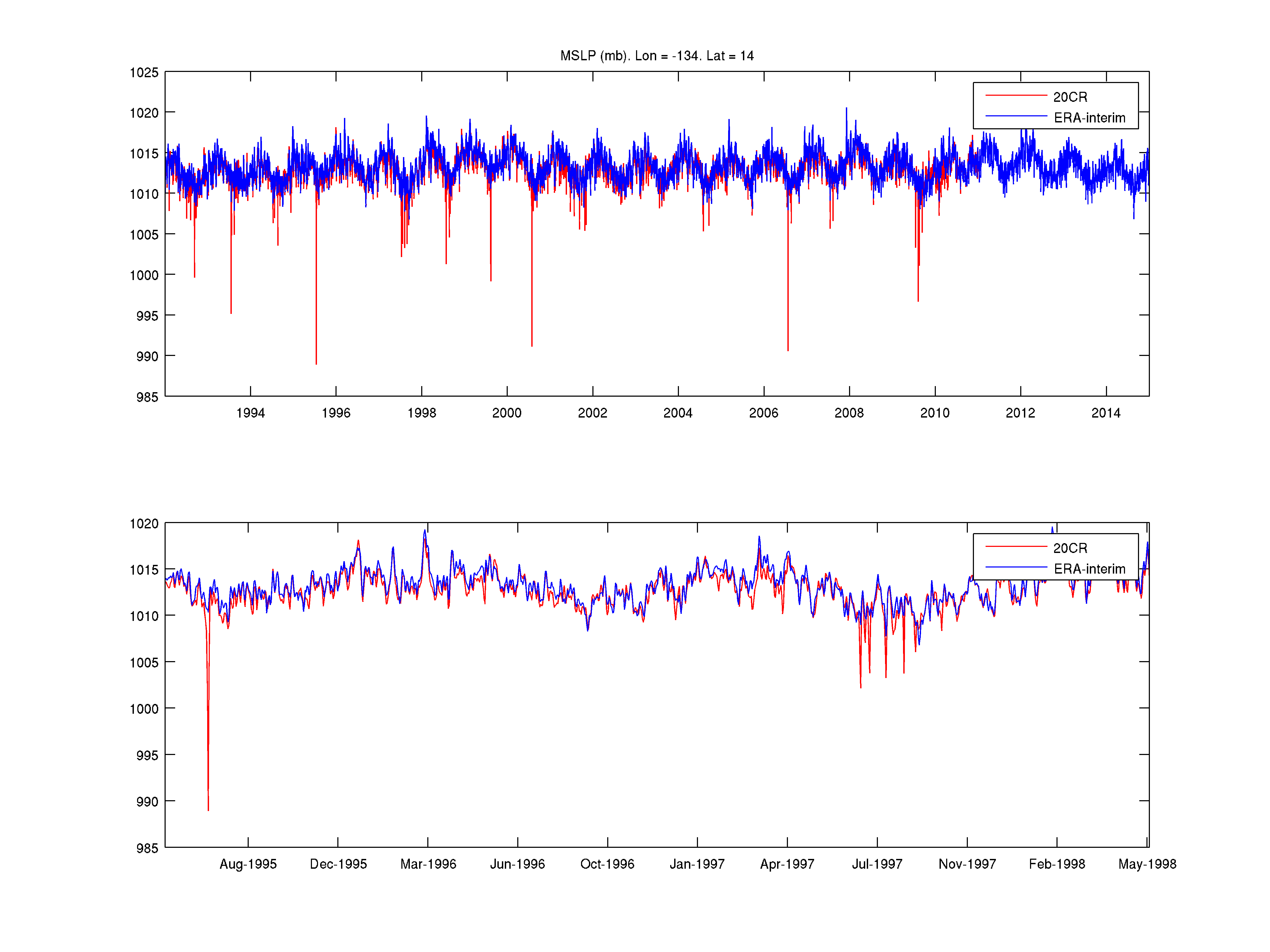
I detected strong drops in the SLP from 20CRv2 not present in the SLP from ERA-interim reanalysis. This happens at some areas, mainly tropical but not exclusively; an example can be seen below for
lon = 134ºW and lat = 14ºN (lower panel is just a zoom of the upper panel). As you can see, differences between both databases can reach 20 mb.
I am using 6-hourly values from both datasets. ERA-interim was downloaded from http://apps.ecmwf.int/datasets/data/interim-full-daily/
and 20CRv2 was downloaded from http://www.esrl.noaa.gov/psd/cgi-bin/db_search/DBListFiles.pl?did=108&t…
Does anybody know if there is a phisical explanation for those drops or if they are outliers?.
Thanks,
Alba
Re: SLP drops in 20CR not present in ERA-interim reanalysis
Dear Dr. Cid,
As noted in the paper Compo et al. (2011, dx.doi.org/10.1002/qj.776) , 20CR version 2 assimilates pressure reports from the International Best Track Archive for Climate Stewardship (IBTrACS, versions denoted in paper). Whether 20CR is "better" is a scientific question that would need further research for you to draw your own conclusions.
Please let me know if I can be of more help.
best wishes,
gil compo
Re: SLP drops in 20CR not present in ERA-interim reanalysis
Have you checked the dates of known tropical cyclones?
Add new comment
Wondering why abrupt PNA shift evident in the Leathers and Palecki (1992) PNA is not apparent in semi-current (as of Oct 2009) NCEP NCAR reanalysis data (Part II)
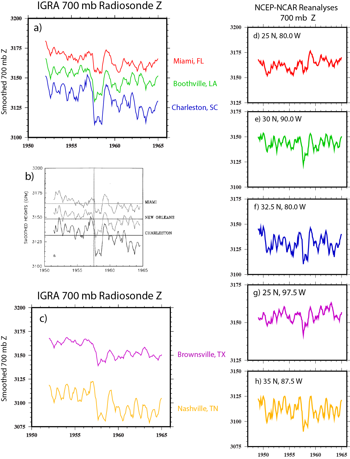
In Part I of this ongoing series ( see 'Wondering why abrupt PNA shift evident in the Leathers and Palecki (1992) PNA is not apparent in semi-current (as of Oct 2009) NCEP NCAR reanalysis data (Part I)') my collaborator and I were trying to figure out why an abrupt shift in the PNA index in ~1957 pointed out by Leathers and Palecki (1992) (hereafter LP92) using older NMC reanalysis data was not found in more recent NCEP-NCAR reanalysis data. The main reason for this is that an abrupt drop in 700 mb Z over the southeastern U.S. (SEUS) that drove that PNA shift was evident in the NMC analysis, but not the NCEP-NCAR analysis. (see LP92's Fig1d and our Fig. 3d in Part I). To look at this more closely we decided to compare IGRA radiosonde variability ( http://www.ncdc.noaa.gov/oa/climate/igra/ ; Durre et al. 2006) for a number of SEUS stations during 1951-1965 with NCEP-NCAR 700 Z series at nearby grid locations.
LP92 had looked at 700 mb Z variability derived from sonde data form New Orleans, Miami, and Charleston SC in their paper (see Fig 1b below), so we downloaded those station's data and data from a number of other SEUS stations. We averaged the IGRA daily data into monthly values, and subjected the monthly 700 mb Z from the IGRA and NCEP data to the same 13 month running average used in LP92. Comparing Fig1a below with Fig1b below shows that our Z series and their Z series for New Orleans, Miami, and Charleston are nearly identical. But while there is a downward shift in 700 mb Z after 1957 that LP92 show as a shift to below mean values in Fig 1b, that same shift is not evident in the NCEP Z series at nearby grid locations in Fig 1d,e, and f. For example, the NCEP Z series in Fig 1d has an upward trend after 1957, while the Miami sonde data in Fig 1 has a downward trend.
The differences between the sonde records for Brownsville TX and Nashville TN (Fig. 1c) and Z variation at the corresponding NCEP grid locations (Fig. 1g,h) are more obvious. Both of the sonde records show a clear regime shift to lower Z values after 1957 that is absent in the reaanalysis Z traces. Otherwise, the IGRA and NCEP trace are similar. For example, if you closely compare the IGRA Brownsville Z trace in Fig. 1c with the Fig. 1g NCEP Brownsville trace you see they closely similar, but that the NCEP values after 1957 are translated upwards. A similar translation also seems evident in the New Orleans, Miami, and Charleston NCEP Z traces (Fig. 1 d,e,f) , but is particularly clear in the Nashville IGRA and NCEP Z series (Fig 1c, Fig 1h).
It seems - and this is just a guess on our part - that NCEP Z values in the southeast US may have been nudged toward climatology after 1957. But this adjustment does not seem consistent with the downward trends and shifts in Z after 1957 in the sonde data. On the other hand, this shift is evident in the older NMC analyses (See LP92's Fig 1d in Part I).
Durre, I., et al. (2006). "Overview of the Integrated Global Radiosonde Archive." Journal of Climate 19(1): 53-68.
Figure 1
Add new comment
Wondering why abrupt PNA shift evident in the Leathers and Palecki (1992) PNA is not apparent in semi-current (as of Oct 2009) NCEP NCAR reanalysis data (Part I)
A collaborator and I have a paper in the Journal of Climate under review that (indirectly) involves the use of NCEP-NCAR reanalysis data. The problem is that we've come across a disagreement between the NCEP-NCAR reanalysis and an older reanalysis used by Leathers and Palecki (1992) and were wondering, basically, which one is right.
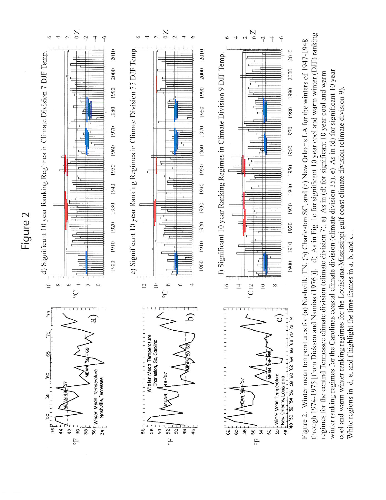
Our paper uses an approach to times series analysis that involves sampling data rankings over moving time windows . I won't go over the details of the method here (see, e.g., Mauget et al. ( 2012)), but in the paper it detected an abrupt regime shift in temperature over the eastern U.S. in the late 1950's. In the paper we show this shift in two Figures (see Figs. 1d and 2d,e,f ). This shift was also noted years ago by Namias (1972) , and Dickson and Namias (1976), so we also included figures from those two papers in our paper for comparison (see Figs. 1c and 2a,b,c ).
Figure 1
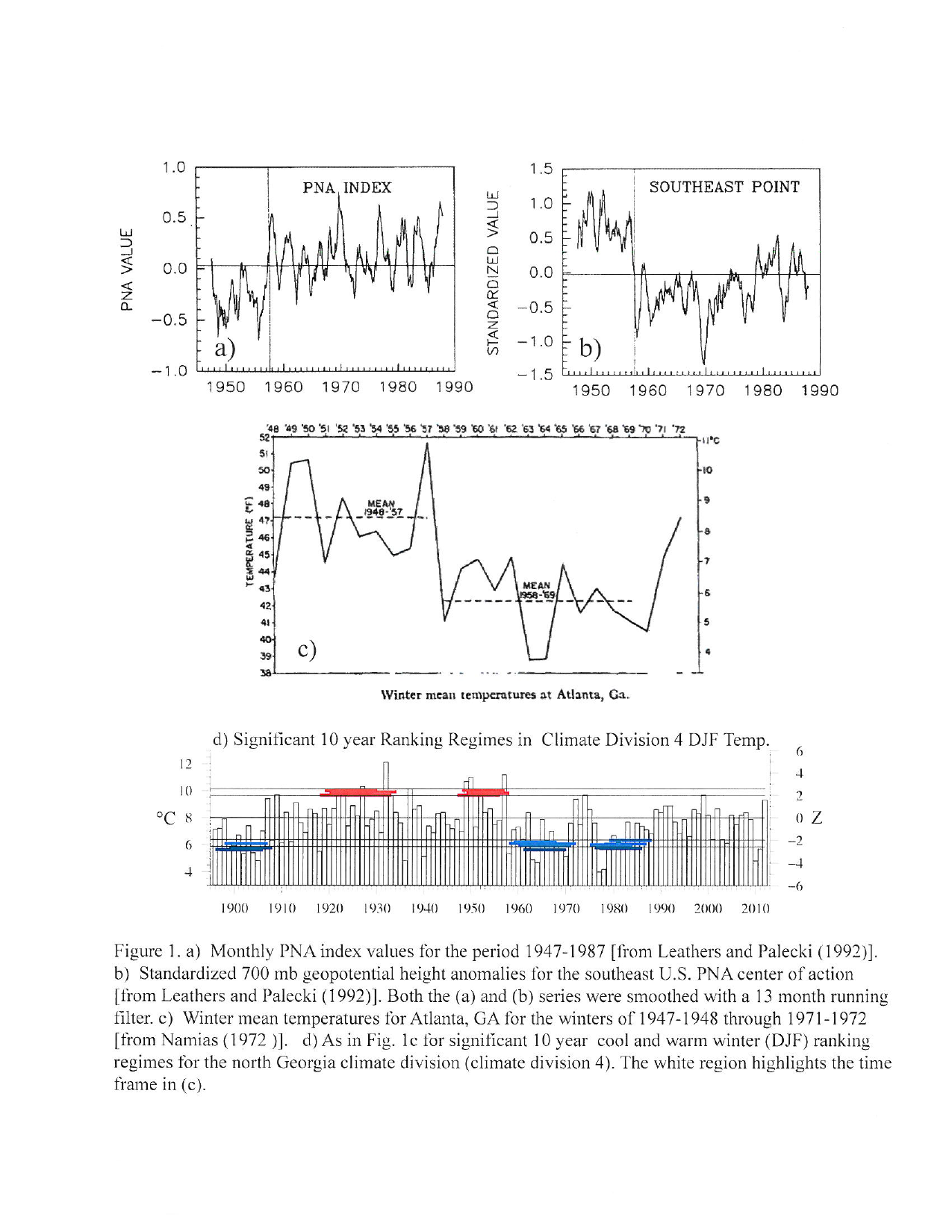
Figure 2
At the same time this shift to colder eastern U.S.temperatures was evident in the late 1950's, Leathers and Palecki (1992) noted an abrupt shift to positive PNA index values. This PNA shift was driven mainly by an abrupt drop in geopotential heights over the southeastern US around 1957. Since that decadal downward regime shift in 700 mb Z was consistent with the eastern U.S. cooling shift that Namias(1972) and Dickson and Namias(1976) noted, we included figures from Leathers and Palecki (1992) that illustrated that PNA and 700 mb Z shift (see Figs. 1a,b).
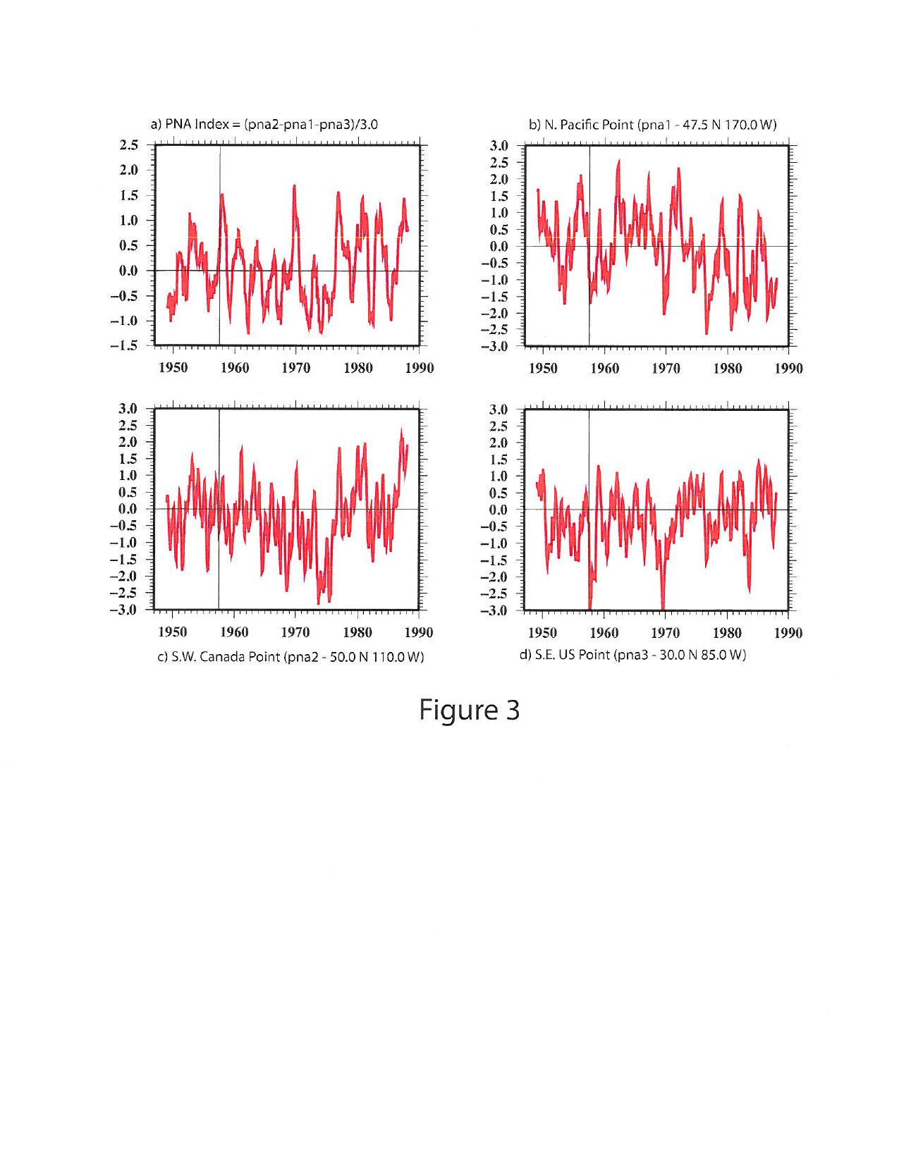
We sent the paper out to be reviewed, and one of the reviewers suggested that instead of showing the Leathers and Palecki (1992) results, we generate our own series for the PNA and the PNA centers of action from more recent data. So I generated those series from the NCEP-NCAR I reanalysis 700 mb Z data I had on hand, which ended in October 2009. I followed the same procedures for generating the series that was outlined in Leathers et al. (1991), i.e., 13 month running filter etc. Afterwards I compared my PNA index with a similarly filtered PNA index derived from the CPC's monthly PNA values. Both correlate pretty highly (r=.918), even though the CPC PNA is derived from Z anomalies at 4 centers of action and the Leathers et al. (1991) PNA is a 3 point index. So I'm fairly sure no dumb mistakes were made.
When you compare the Leathers and Palecki (1992) results and and our similarly organized PNA series in Fig. 3 below you can see that the abrupt PNA shift evident in the Leathers and Palecki PNA is not found in the current NCEP NCAR reanalysis data. This is mainly because the drop in 700 mb Z over the southeastern US in ~ 1957 that is evident in Leathers and Palecki's results (their Fig. 1d) is not evident in the reanalysis data we're using (our Fig. 3d).
Leathers and Palecki (1992) Fig.1
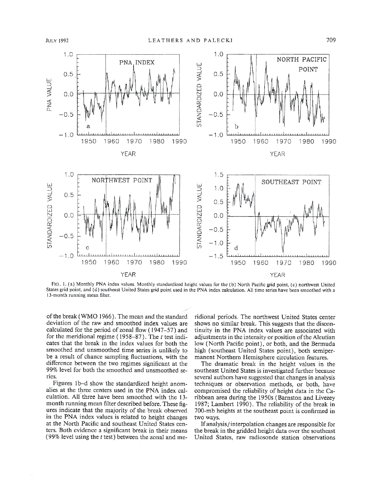
Figure 3
I always thought that the southeastern U.S. shift in 700 mb Z shown in Leathers and Palecki (1992) (Their Fig. 1b) seemed kind of exaggerated. On the other hand, it is completely absent in the NCEP-NCAR reanalysis even though our analysis and those of Namias (1972) and Dickson and Namias (1976) show a decadal shift to cooler temperatures over the southeastern U.S. during the 1960's. My guess is that kind of persistent shift to cooler temperatures would also lead to some kind of drop in lower atmosphere Z, but there is no trace of that in the NCEP-NCAR data.
So our question is: Why is this drop in geopotential clearly evident in the Leathers and Palecki PNA index - which was derived from NMC daily 700 mb octoganal grid analyses - but not apparent in NCEP-NCAR 700 mb Z? Could this late 1950's geopotential shift may have been identified as a spurious feature in the NCEP-NCAR reanalysis and adjusted out somehow? Was the shift in the Leathers and Palecki (1992) seen as some kind of reanalysis artifact, or a consequence of a shift in the radiosonde data? They consider this possibility in Leathers and Palecki (1992), but show similar shifts in radiosonde Z and surface temperature over the southeastern U.S.
I've taken a look at the reanalysis problems list at http://www.esrl.noaa.gov/psd/data/reanalysis/problems.shtml. I see that the daily times that data was collected changed in 1957 – about the same time we see the 700mb Z shift in Fig. 1b - but other than that I don't see anything related to this problem. Does anyone at Reanalyses.org have any ideas on this?
References
Dickson, R. R. and J. Namias (1976). "North American Influences on the Circulation and Climate of the North Atlantic Sector." Monthly Weather Review 104(10): 1255-1265.
Leathers, D. J., et al. (1991). "The Pacific/North American Teleconnection Pattern and United States Climate. Part I: Regional Temperature and Precipitation Associations." Journal of Climate 4(5): 517-528.
Leathers, D. J. and M. A. Palecki (1992). "The Pacific/North American Teleconnection Pattern and United States Climate. Part II: Temporal Characteristics and Index Specification." Journal of Climate 5(7): 707-716.
Mauget, S. A., et al. (2012). "Evaluating Modeled Intra- to Multidecadal Climate Variability Using Running Mann–Whitney Z Statistics." Journal of Climate 25(5): 1570-1586.
Namias, J. (1972). "Experiments in Objectively Predicting Some Atmospheric and Oceanic Variables for the Winter of 1971–72." Journal of Applied Meteorology 11(8): 1164-1174.
Re: Wondering why abrupt PNA shift evident in the Leathers ...
I don't have an answer but I have some comments. Your PNA index is based on 3 points which are in the North Pacific, SW Alberta and in the Gull off Alabama. If you plot the upper data (adupa, sondes + pibals) using
http://nomad1.ncep.noaa.gov/cgi-bin/pdisp_r1_obs.sh
you can see the upper air data in the late 1950s. The North Pacific is poorly covered. The other two points are near the CONUS so their quality would be better than no nearby stations but worse than if they in the CONUS. So their is some concern about the accuracy of the PNA index. Perhaps you should define your own PNA index and put the 3 points on top of long-term rawinsonde stations like in the Aleutian Islands.
Leathers et al found a discontinuity in the Z700 around 1957 (fig 1b). Now IGY (International Geophysical Year) was in 1957-1958 and the launch times for radiosondes were standardized to 00Z and 12Z. A change in the launch times could create a break in the Z700 as seen in fig 1b if the analysis scheme did not account for the diurnal cycle. (I would be surprised if the old analyses accounted for the diurnal cycle because where would they get the diurnal cycle data?) On the other hand, the NCEP/NCAR Reanalysis (R1) should be insensitive to the launch times because the diuranal cycle is generated by the forecast model. There will be some sensitivity to the launch time because the model has an imperfect diurnal cycle. The next step would be to figure out the launch times. I didn't find it with google, so have to look at the bufr files.
Re: Wondering why abrupt PNA shift evident in the Leathers ...
Wesley:
Thanks for your comments. I'm not so much concerned about the overall PNA variability as much as I am the 700 mb variation over the southeast U.S.(SEUS) PNA center of action. Leathers and Palecki (1992) actually addressed skepticism about the 1957 SEUS 700 mb Z drop by making two points.
First, they demonstrated that the regime shift in Z was present in the rawinsonde data (Their Fig. 2a), so they reasoned that it couldn't be due to some change in the analysis procedures.
Second, they noted the change in observation times during the 1957-58 IGY, which basically moved the twice daily obs backward from 1500 & 0300 Z to 1200 & 0000 Z. However, after presenting evidence of an abrupt shift in SEUS temperature regime regime (their Fig. 2b), they reasoned that the shift was due to the change in surface forcing and not the change in observation times. I'm not sure I completely buy their logic on that, but I still think that their Fig. 1d SEUS Z drop was due to surface forcing for two reasons. First, if the change in observation times had that effect in the SEUS PNA center of action ,why didn't it have a similar effect on the southern Alberta center of action (their Fig. 1c)? Second, I'm not that familiar with how rawinsonde data is processed, but I assume the twice daily measurements are averaged to remove daily Z variation. Would changing twice-daily upper-air obs by 3 hours have that much of an effect on the daily average Z height measurement? Leather's and Palecki's Fig. 1d, which shows the normalized 700 mb Z drop, has Z dropping by ~ 1 standard deviation. Although I can't prove it, my guess is that was not due to a relatively minor shift in observation times.
My hunch, which doesn't pull much weight with most reviewers, is that the 1957 SEUS 700 mb Z drop in Fig. 1d was real. But I have no idea why its not apparent in the NCEP-NCAR 700 mb Z reanalysis data.
Thanks again for you input,
Steve M.
Re: Wondering why abrupt PNA shift evident in the Leathers ...
Dear Steven,
You may want to look at the 20th Century Reanalysis data (http://go.usa.gov/XTd ). 20CR only uses pressure observations. A version of the PNA series is shown in Compo et al. 2011 http://dx.doi.org/10.1002/qj.776 .
You can compare each center of action with NCEP-NCAR reanalsis using the WRIT timeseries tool or look at maps
https://reanalyses.org/atmosphere/writ , in addition to downloading the data for your own analysis.
The NMC analyses had many discontinuities. One of the main reasons to perform reanalysis with the same model and assimilation method is reduce discontinuities that arise from changing methods (see references in Compo et al. 2011 for a detailed discussion of this point). The Kistler et al. 2001 BAMS paper talks about some of the radiosonde corrections.
Given the changes in the radiosonde and global observing network associated with the International Geophysical Year in 1957 and 1958, any shifts in original analyses in particular, have to be treated cautiously.
Please let me know if I can be of any additional help.
best wishes,
gil compo
Re: Wondering why abrupt PNA shift evident in the Leathers ...
Gil:
Thanks a lot… those are all very helpful suggestions. I've downloaded your 20Cr paper and the Kistler paper and I'll see what information they provide.
Steve Mauget
Add new comment
GOAT (Geophysical Observation Analysis Tool)
GOAT (Geophysical Observation Analysis Tool)
Analysis:
GOAT archives all geophysical data in a consistent format, thereby reducing the need to bother with the esoteric details of the particular datasets.
GOAT icludes a GUI based interface for intuitive browsing, subsetting and display of data in all spatial and temporal projections.
The GUI also provides some advanced analysis features such as:
- Calculation of climatology and anomalies
- Spatial and temporal filters
- Display differences between two fields
- Display superposition of two fields
- Include topography in display or analysis
- Code generation (similar to the 'Generate Code' option in MATLAB figures)
Data retrieval:
GOAT intgrates with OPeNDAP sources and NetCDF files via a process referred to as 'linking' (GOAT LINK Format). GOAT also integrates with *.mat file archived in a GOAT standard format (GOAT MAT Format). The GOAT GUI also enables converting linked OPeNDAP and NetCDF archives to MAT Format. Information on GOAT archiving formats can be found in the GOAT documentation.
OPeNDAP sources (GOAT LINK Format):
LINK archives do not require much disk space (typically a few MB per archive). A full list of available OPeNDAP LINK archive can be found here. Examples of available OPeNDAP LINK archives are
- MERRA (entire archive)
- 20th Century Reanalysis (entire archive)
- NCEP I and II (entire archives)
- ERA-40 (partial archive)
- ERA-Interim (entire archive. Uses a specially designed perl based protocol for communicating with the MARS server)
- ORA-S4 ocean reanalysis.
NetCDF files (GOAT LINK Format):
GOAT indludes functions for automatically linking NetCDF files following the CMIP5 standard. In particular, the GOAT_CMIP5_LINK function (which can also be launched from the GOAT GUI) automatically finds all CMIP5 files in a specified folder and creates LINK archives for these files.
This functionality can be further extended to other datasets as a growing number of observational datasets are now available in CMIP5 archiving standard via the obs4MIPs and ana4MIPs projects.
Conversion of datasets to *.mat files (GOAT MAT Format)
GOAT includes a GUI based data download tool for automatically downloading and converting datasets to GOAT MAT Format (*.mat files).
Information on available datasets for download can be found here.
The following datasets are available via the GUI based tool:
Atmosphere
Clouds
- CloudsatCalipso (a combination of Cloudsat and Calipso by Jennifer. E. Kay)
Surface
Ocean:
Re: GOAT (Geophysical Observation Analysis Tool)
can I get the land mask of Siberia region and Himalayan region?
Re: GOAT (Geophysical Observation Analysis Tool)
that would depend on the dataset . . .
one crude way of deriving such a mask in GOAT would be to spatially truncate an ocean surface field in the region you are interested in, save it, and set Nans to 1 (land) and non-Nans to 0 (ocean) in the saved field.
Re: GOAT (Geophysical Observation Analysis Tool)
The NCAR Research Data Archive serves numerous reanalysis datasets, many of which should have the land-sea mask stored in their 'constant' or 'fixed' fields. Usually it's stored as a grib record. Go to http://rda.ucar.edu/, and go to 'Atmospheric Reanalysis Data' under the header 'Other ways to explore'. Each reanalysis dataset has the e-mail contact listed for the data specialist who manages the dataset. Please e-mail the specialist if you are unable to find the land mask data.
GOAT access to 20CR every member data?
Does GOAT already include or will it include access to the 20CR OPeNDAP enabled every-member data in netCDF4 format at
in the analysis, analysis.derived, first_guess, and first_guess.derived directories?
subdaily, daily-averaged, and monthly-averaged every member fields are available there.
best wishes,
gil
Re: GOAT access to 20CR every member data?
Not at present.
In a few weeks a new version of GOAT will be released which includes OPeNDAP access to the entire MERRA archive, and other reanalyses with OPeNDAP access.
20CR is one of the reanalyses on the list.
It will also be possible to link GOAT to the native *.nc files of an existing (i.e. not via OPeNDAP) CMIP5 archive.
Ori.
Re: GOAT access to 20CR every member data?
The latest version of GOAT (2014E) includes access to 20CR OPeNDAP enabled data (mean and spread but not every-member data) and some other datasets with OPenDAP enabled data.
Add new comment
Trends in reanalysis data sets
Hello. This is my first correspondence on this forum. Forgive me as I haven't used WIKI for quite a few years and need to re-educate myself.
I dabbled in some reanalysis data a few years ago and had little to do with it regularly until a few months ago. I am very impressed with the progress made, not that I knew much about it all beforehand, and warmly compliment all involved. The free access to this wonderful resource coupled with the opportunities freely available packages such as 'R' allow to one to 'play' with the data, make it a fun opportunity for enquiring minds to understand and educate others in this fascinating subject.
The main reason I drifted back to this resource was because of the paper 'Evidence linking Artic amplification to extreme weather in mid-latitudes' by Jennifer Francis and Stephen Vavrus. They used the reanalysis data in their paper.
http://www.vliz.be/imisdocs/publications/234818.pdf
In locating this URL I stumbled across this piece that appeared on the Internet just today, so the research is understandably worthy of attention given what is going on with the world's weather.
http://www.nzherald.co.nz/gwynne-dyer/news/article.cfm?a_id=153&objectid=11204955
However I would strongly urge anybody interested in this important issue to visit the page:
http://www.abc.net.au/catalyst/stories/3796205.htm
You can read the narrative, watch the episode and even download a copy. It's a good summary of what issues are importantly at play with regards to climate change and Francis's research is considered at the end of it.
The reason for my correspondence here deals with the fact that I downloaded some reanalysis data to have a look at the issue myself. Unfortunately I stumbled across some data I was uncomfortable with. For various reasons I'm not the most motivated person when it comes to writing up my calculations and my short private correspondence on the matter died. I then found this website, so I thought I might try this avenue if you don't mind. I'll try and keep it to a minimum and make the data and 'R' code I have used available to others to re-produce, correct and add to, if there is an interest. If done correctly and in the right spirit it might be a good opportunity to help educate some folks who are starting out on a journey to explore the endless opportunities that exit with this resource. Especially as the data set deals with the world and we can all learn from others experiences with the circumstances elsewhere.
As a starter, I downloaded annual daily temperatures for the world [144 x 73 grid points] from the US reanalysis I data set for the years 1980-2012. From this, I used 'R' to compute the annual average values for each grid point and I have saved into a netCDF3 file which I will gladly make a link to, if anybody wants a copy to look into this data themselves and doesn't want to re-do what has already been done. The first thing I was interested in was to derive a simple linear regression between the annual temperatures and the year for all grid points, to gauge what % of grid points are rising and falling. I decided to plot the regression slope against the correlation so that I could get an idea of the size of the trend and the strength of the trend (as measured by the correlation). The plot I obtained was:
http://home.iprimus.com.au/davejwil/tsfc_annual_correl_slope.png
I was rather taken by the plot. The majority of the points lay in the top right of the plot signifying a rising trend in the values, which is what I expected, but the size of some of these and particularly a few of the falls, are surely too large. The annual slopes range from -0.2852 to 0.2089. When multiplied by 32 to account for the 32 year period of the data, this comes to -9.1 to +6.7 deg changes over just 1/3 of a century. Further exploration is in order.
I won't say anything more for the moment but have obtained EC and US2 data sets for the area where the temperature falls are notably contrary to the rest of the data set. These apply to the mountainous region of South America. The most significant decline here occurs at the grid point 70W, 30S and the figure below shows how it arose.
http://home.iprimus.com.au/davejwil/tsfc_70W_30S.png
In concluding this contribution, I've listed the values below for anybody who wishes to have a 'play'. If you average the values from 1980-1998, it means 9.92 with a standard deviation of just 0.47; its very consistent. For the period 1999-2012 the average drops to 3.96 with a standard deviation of 1.43. A t-test on these 2 series, assuming an unequal variance, gives a t-value of 15 and a 95% CI of the difference as [5.11,6.81]. Clearly there is something at play here and it isn't climate related. I will discuss this further in subsequent correspondence if it is OK to do so.
I would also like to point out that I'm also dabbling in some 'perfect prog' calculations on rainfall probabilities in Australia using the reanalysis data set. The results very nicely connect the indicence of rain [we don't get snow here much...] with basic atmospheric conditions and the data analysis would be of some interest to those folk who have ventured to this wonderful resource and would like to get a feel for what absorbing things they could do with it.
Regards
Dave
1980 9.5
1981 9.7
1982 10.8
1983 10.2
1984 9.9
1985 10.3
1986 10.8
1987 10.1
1988 9.3
1989 9.8
1990 9.6
1991 9.9
1992 9.4
1993 9.7
1994 10.4
1995 10.2
1996 9.3
1997 10.2
1998 9.3
1999 6.6
2000 5.0
2001 5.4
2002 4.2
2003 4.1
2004 5.1
2005 4.3
2006 3.1
2007 1.7
2008 2.6
2009 2.9
2010 2.1
2011 3.0
2012 5.3
Add new comment
Temperature trends for the period 1871-2009 in the midlatitude summer mesosphere
Lübken, F.-J., U. Berger, and G. Baumgarten (2013),
Temperature trends in the midlatitude summer mesosphere,
J. Geophys. Res. Atmos., 118, doi: 10.1002/2013JD020576.
A trend analysis of long term runs have been performed with the LIMA model (0-150 km altitude) applying the NOAA-CIRES 20th Century Reanalysis (V2) from 2009 back to 1871. LIMA adapts the Reanalysis data (u,v,T) with global coverage every 6 hour below about 25 km applying a nudging method. Variations of green house gases CO2 and O3 have been predescribed according to observations. Trends have been estimated in the troposphere, stratosphere, and mesosphere at mid-latitudes for summer conditions (June - August).
As a main result trends are non-uniform with time.
Since the late 19th century, temperatures in the mesosphere have dropped by up to 5-7 K (10-12 K) on pressure (geometric) altitudes.
This is much more than typical trends in the troposphere and stratosphere. The summer mesosphere therefore reacts much more sensitive to climate change compared to lower altitudes.
Short summary:
In Fig. 1 we show mean June to August temperatures at 54°N from LIMA at geometric height of 70 km based on NOAA-CIRES 20th Century Reanalysis. We have performed a multivariate fit based on three functions (also shown in Fig. 1), namely CO2(t), O3(t), and Ly-alpha(t). The largest contribution to the long term temperature trend comes from CO2, whereas O3 has an impact in the last 30 years only (by construction), and Ly-alpha(t) causes a quasi-periodical modulation. Obviously, temperature trends are not uniform in time but accelerate since approximately the 1960s. Comparison with CO2(t) clearly shows that this acceleration is due to an increase of carbon dioxide. We have calculated temperature trends in three periods, namely from the beginning of the time series (1871) to 1960, from 1960 to present time (2008), and over the entire period. The results are shown in Fig. 2. As expected, trends are larger in the second period. In pressure coordinates, total temperature trends are largest in the upper stratosphere and mesosphere, more precisely at 40-70 km. Trends are minimal around the mesopause. In geometric heights, trends are generally larger and, for the second period 1960-2008, clearly maximize in the mesosphere, where trends can be as large as -1.8 K/dec. We note that this trend analysis produces very similar results in comparison with a detailed trend analysis using ECMWF reanalysis data in the period 1961-2009 (for more details, see Lübken et al, JGR, 2013).
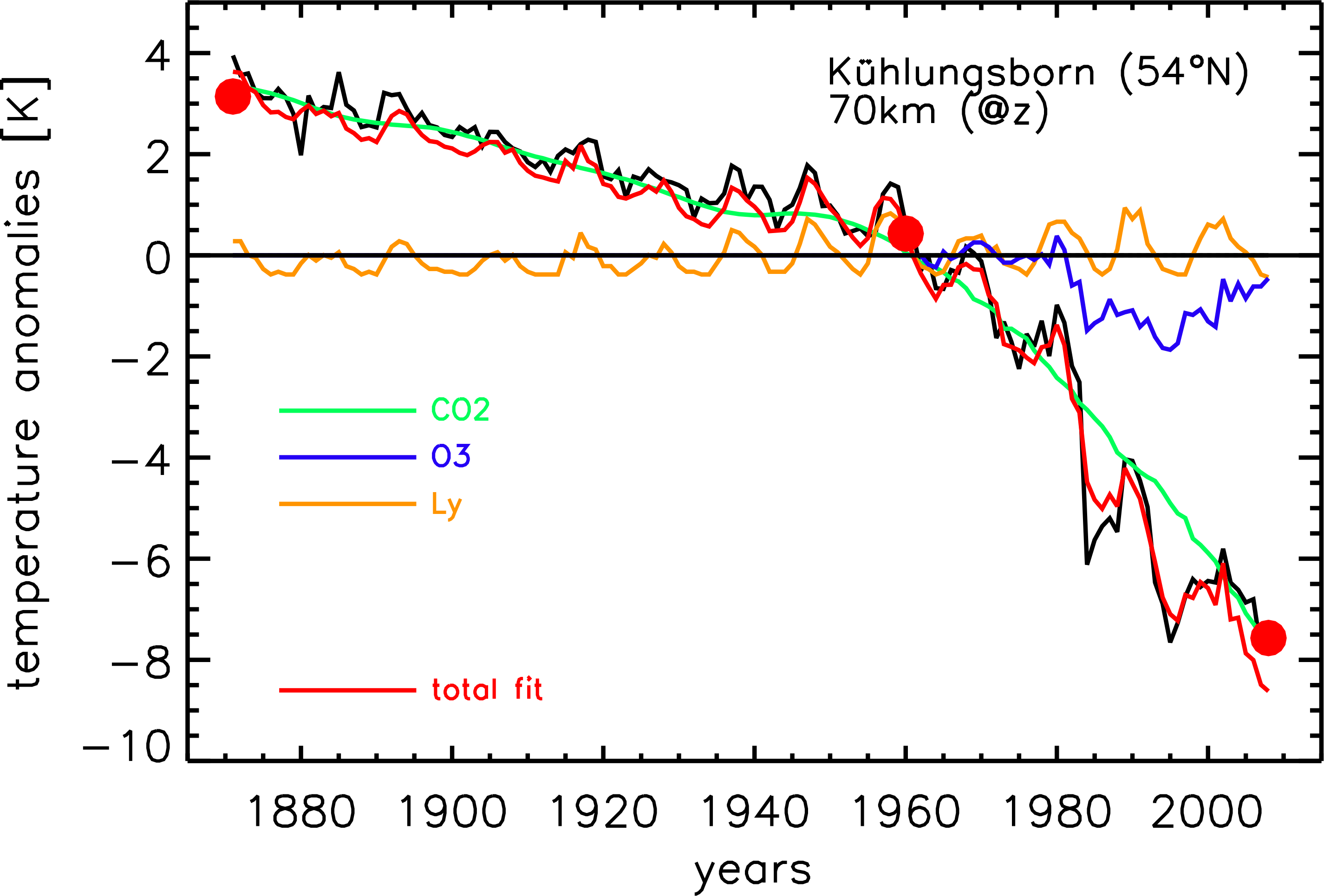
Fig.1: Temperature anomalies (=deviations from the June-August 1871-2009 mean) at zgeo=70 km at 54°N (Kühlungsborn, Germany) from 1871 to 2008 (black line). The result of a multivariate fit (red) consisting of CO2(t) (green), O3(t) (blue), and Ly-alpha(t) (orange) is also shown. Temperatures are marked at the beginning and at the end of the time series, and around 1960 where the trend changes markedly (red dots).
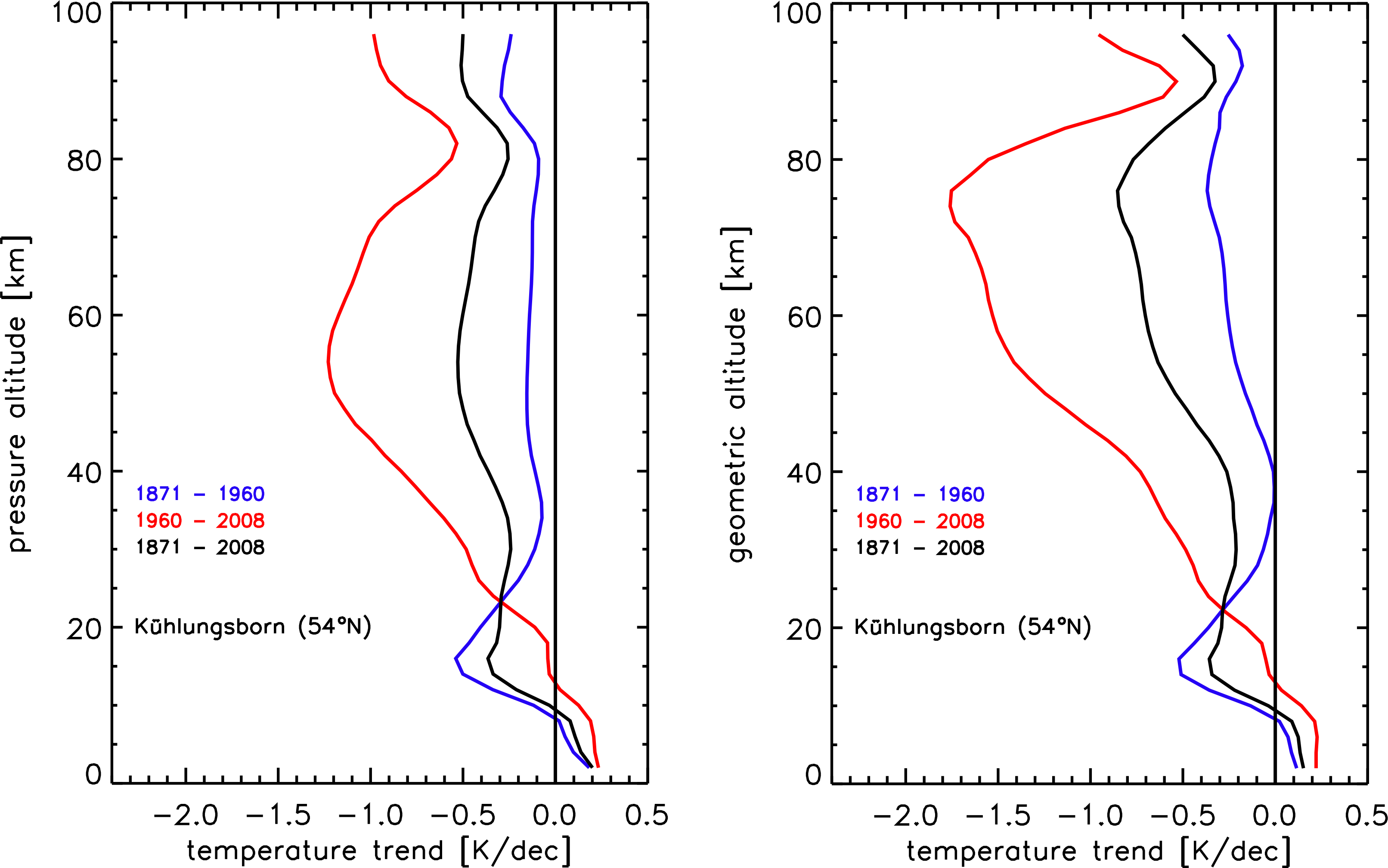
Fig.2: Temperature trends (June-August) for the location of Kühlungsborn 54°N) as a function of pressure (left) and geometric (right) altitudes. Black lines show the trend over the entire period (1871-2008), whereas blue and red lines show trends in the subperiods 1871-1960 and 1960-2008, respectively.
Potential biases from 20th Century Reanalysis nudging?
Dear Dr. Lübken,
Very interesting! Looking at your paper, I don't see how the temperature biases in the 20CR stratosphere were handled.
(see, e.g., Fig. A1 in Compo et al. 2011, (available at http://onlinelibrary.wiley.com/doi/10.1002/qj.776/abstract ) Do you think that the biases might have an impact on your results?
Also, how similar are the trends in the latter period to your results using ECWMF reanalyses in your paper Fig. 10?
best wishes,
gil compo
U. of Colorado/CIRES & NOAA Earth System Research Laboratory
Add new comment
20CR: ensemble mean wind-speeds appear wrong
I suspect that the 20CR.v2 ensemble mean wind speeds provided publicly were calculated incorrectly, and I will briefly explain.
As confirmed in the attached plots, the ensemble mean speeds provided for 20CR were computed as:
wspd = [<u>^2 +<v>^2]0.5
where <> indicates the ensemble mean. The correct calculation would be
wspd = < [u2 + v2]0.5 >
As you can see in the attached, the provided ensemble mean speeds look nothing like the speeds in the individual ensemble members, and appear wrong.
After downloading all the individual ensemble members and recalculating the speeds using the correct formula above, I get an ensemble mean which is perfectly
consistent with the individual members (i.e. falls in the middle of them), as would be expected.
The ensemble mean wind speeds provided also look physically unrealistic (e.g. too low at extratropical latitudes prior to the 1990's), and exhibit unrealistically
large trends. When using the individual ensemble members, or the correctly re-calculated ensemble mean speed, these issues are corrected.
I suspect many users could be affected by this, and I hope that this info might be useful.
-Neil Swart
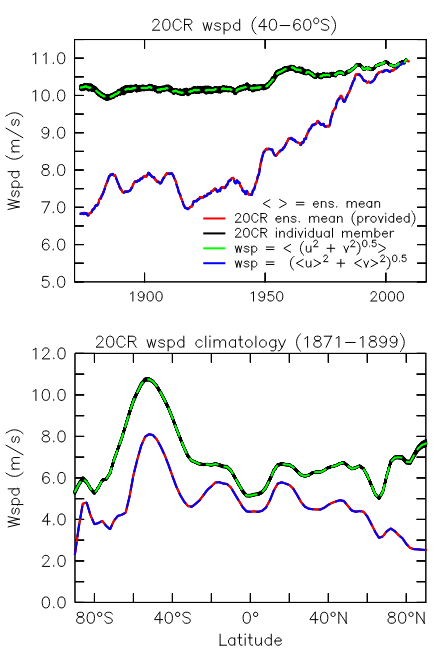
Note in the time-series plot attached the data are all smoothed with a 5-year wide boxcar.
Land mask for 20CRV2c rectangular 2x2 grid
Is there somewhere a file with a land mask for the 20CRv2c 2x2 rectangular grid (91x180) ?
I only found the land mask for the gaussian grid (94x192).
Thanks in advance. Claude
Re: Land mask for 20CRV2c rectangular 2x2 grid
Claude,
The land mask is only used by the first-guess. Those fields are generated on the gaussian grid (94X192), so the land mask is available on the gaussian grid.
Any other field will be an interpolation. You are welcome to use your favorite method to do the interpolation.
best wishes,
gil
Re: 20CR: ensemble mean wind-speeds appear wrong
I also have a question:
Can you confirm whether this issue might affect the wind-stress fields too?
I.e.: Calculating the ensemble mean stress as
tauu = ^2
instead of
tauu = < u^2 >
Or are the stess fields computed online in the model from the instantaneous U and V and therefore okay?
Re: 20CR: ensemble mean wind-speeds appear wrong
**Should have read
tauu = \^2
instead of
tauu = < u^2 >
Re: 20CR: ensemble mean wind-speeds appear wrong
Neil,
The issue should not affect the wind stress. They are computed for every member and then averaged.
Please let us know if you find something different.
best wishes,
gil
Re: 20CR: ensemble mean wind-speeds appear wrong
Hi Gil,
In these calculations using all the individual ensemble memebers I was only considering the sigma .995 level winds. I have also looked in some detail
at the 10 m winds - at least at the ensemble mean 10m winds downloaded from ESRL. My guess is that the same issue affects the 10 m wind
speeds, because they also exhibit the (unrealistically) large trends in time, as seen in the sigma .995 winds above.
That said, I cannot confirm this by performing the same calculation with the 10m winds, because the individual ensemble members for the 10 m winds
are not available on the nersc.gov site, as far as I can see.
-Neil
Re: 20CR: ensemble mean wind-speeds appear wrong
Neil,
10 m winds are at the portal.nersc.gov site in netCDF4. They are under the "first_guess" directories. For example, for the 10 m zonal wind
http://portal.nersc.gov/pydap/20C_Reanalysis_ensemble/first_guess/u10m/
These are also OPeNDAP enabled.
The "derived" directories at
http://portal.nersc.gov/pydap/20C_Reanalysis_ensemble/
have the daily and monthly averages for each member.
Additional selected variables are available from the NERSC Tape Science Gateway in GRIB format:
http://portal.nersc.gov/archive/home/projects/incite11/www/20C_Reanalysis/everymember_grib_indi_fg_variables
and 3 dimensional and surface grids in GRIB format for most years at
http://portal.nersc.gov/archive/home/projects/incite11/www/20C_Reanalysis/everymember_full_analysis_fields
Note that the first guess is not directly incremented by the observations. It is the product of the numerical weather prediction model forecast initialized from the analyzed state.
Please let me know if I can be of more help.
best wishes,
gil
Re: 20CR: ensemble mean wind-speeds appear wrong
Neil,
Thanks for pointing this out. What level are you examining? Are these the 10 m winds?
thanks,
gil compo
Re: 20CR: ensemble mean wind-speeds appear wrong
Hi Cathy,
Thats good to know, thanks. The resulting wind-speed errors are not small, but in fact are very large (>3m/s or 50% in some cases).
You can see that very clearly in my figure - but I'm having trouble getting that to show up in the post. SOrry but I'm a noob at editing these pages!
Re: 20CR: ensemble mean wind-speeds appear wrong
We will look at calculating the values from the individual ensemble members. You are correct the wind speed from the ensemble means would be lower than that of the average wind speed of the ensemble members and it would be most different where the ensemble members were most different from each other.
We don't have the wind speed file listed in our docs but it is in /Datasets/
I'll remove the files and document this. I'm not sure when we can generate the re-computed files.
Re: SLP drops in 20CR not present in ERA-interim reanalysis