20CR

How to access preliminary NOAA-CIRES-DOE 20CRv3 data at the National Energy Research Scientific Computing Center (NERSC).

First, you must obtain an account at http://www.nersc.gov/users/accounts/user-accounts/get-a-nersc-account/  .
In the Description field of the account form, enter "I will be working with Gilbert Compo on analyses of the new NOAA-CIRES-DOE 20th Century Reanalysis version 3 using repo m958. I will be studying <your scientific interest goes here>." 

To see details on the model, assimilation, observations, and other implementation algorithms, click here.

Ensemble Mean and spread files in GRIB and text observation files are currently available on disk at NERSC:

/project/projectdirs/incite11/ensda_v451/ensda_[syear]/YYYYMMDDHH and

/project/projectdirs/20C_Reanalysis/ensda_v452/ensda_[syear]/YYYYMMDDHH, where:

• 451 = 20CRv3si and 452 = 20CRv3mo

• syear = “stream year” is any year from 1804 - 2009 ending in a 4 or a 9

• Yearmonthdayhour directories are available every six hours (00,06,12,18)

Within a directory, there are several types of files. Consider the example 1916010100:

> l /project/projectdirs/incite11/ensda_v451/ensda_1914/1916010100

total 234240

drwxrwxr-x     2 cmccoll m958  131072 May 24 14:50 ./

drwxrwxr-x+ 8895 cmccoll m958   524288 Jul 24 17:08 ../

-rwxrwxr-x     1 cmccoll m958 15102002 Jan 11  2018 pgrbensmeananl_1916010100.grb2*

-rwxrwxr-x     1 cmccoll m958 16957694 Jan 11  2018 pgrbensmeananl_1916010103.grb2*

-rwxrwxr-x     1 cmccoll m958 16966630 Jan 11  2018 pgrbensmeanfg_1916010100_fhr06.grb2*

-rwxrwxr-x     1 cmccoll m958 57797749 Jan  3 2018 pgrbenssprdanl_1916010100*

-rwxrwxr-x     1 cmccoll m958 65366796 Jan  3 2018 pgrbenssprdanl_1916010103*

-rwxrwxr-x     1 cmccoll m958 65280022 Jan  3 2018 pgrbenssprdfg_1916010100_fhr06*

-rwxrwxr-x     1 cmccoll m958   90315 Jan 3 2018 psobfile*

-rwxrwxr-x     1 cmccoll m958   88308 Jan 3 2018 psobs.txt*

-rwxrwxr-x     1 cmccoll m958  149856 Jan 3 2018 psobs_posterior.txt*

-rwxrwxr-x     1 cmccoll m958   88977 Jan 3 2018 psobs_prior.txt*
 

“pgrb” refers to grib (for spread files) or grib2 (for mean and everymember files) filetype.

“anl” refers to “analysis”, and “fg” refers to “first guess”. Not all variables are available in all types of files. Accumulated and averaged variables are only available in pgrb files 3 hours after the central analysis time (in this example 00Z) and in the “fg” file valid 6 hours after the central analysis time.  Accumulations and averages are needed from both to make a 3 hourly timeseries. See below for more details.

psob* are each text files with observation statistics; psobs_posterior.txt is the final file with all statistics after completing the assimilation of observations at that time step. See link for specifics regarding each field in this file.

Examples for YYYMMDDHH = 2011010100:

pgrbensmeananl_YYYYMMDDHH.grb2 (pgrbanl, for short)

pgrbensmeananl_YYYYMMDD{HH+3}.grb2  (pgrbanl+3 for short)

pgrbensmeanfg_YYYYMMDDHH_fhr06.grb2  (pgrbfg for short)

Note that grib1 files (ie, ensemble spread files) will have the same variables, but may have different names depending on your reader.

In particular, note that precipitation rate is only in the pgrbfg* and pgrbanl+3. For YYYYMMDDHH = 2011010100 as above, note that the pgrbfg* file actually contains 3-hour average precipitation rate from 2010123121 to 2011010100, and the pgrbanl+3 contains the 3-hour average precipitation rate from  2011010100 to 2011010103.

This holds true for other average and accumulation variables.

Ensemble Mean and spread files in netCDF are currently available on disk at NERSC (to use nc tools run "load module nco")

Yearly files of 3 hourly or monthly mean fields for selected variables are currently being generated in 

/global/cscratch1/sd/cmccoll/ensmean_ncfiles_v451  
/global/cscratch1/sd/cmccoll/enssprd_ncfiles_v451
/global/cscratch1/sd/cmccoll/ensmean_ncfiles_v452  
/global/cscratch1/sd/cmccoll/enssprd_ncfiles_v452
 

As an example, files for Pressure at Mean Sea Level (PRMSL) are available from 1836 to 1980 in v451 directories and 1981 to 2015 in v452

ls /global/cscratch1/sd/cmccoll/ens*ncfiles*_v45?/PRMSL*

/global/cscratch1/sd/cmccoll/ensmean_ncfiles_v451/PRMSL.1836.mnmean_v451.nc
/global/cscratch1/sd/cmccoll/ensmean_ncfiles_v451/PRMSL.1836_v451.nc
...

/global/cscratch1/sd/cmccoll/ensmean_ncfiles_v452/PRMSL.2015.mnmean_v452.nc
/global/cscratch1/sd/cmccoll/ensmean_ncfiles_v452/PRMSL.2015_v452.nc
 

Ensemble Mean and spread files in netCDF available at NERSC’s high performance storage system (HPSS)

To see what is available in a given HPSS directory, login to Cori (or Edison),  and run “hsi ls /home/projects/incite11/[subdirectory]/”

possible subdirectory:

    ensda_v451_ensmean_netCDF

    ensda_v452_ensmean_netCDF

    ensda_v451_enssprd_netCDF

    ensda_v452_enssprd_netCDF

filenames: - VAR_Y1-Y10_ensmean_v451.tar

                    VAR_Y1-Y10_enssprd_v451.tar

        VAR is the variable

         For V451 Y1-Y10 can be 1836-1845,1846-1855,1856-1865...1976-1980

         For V452 Y1-Y10 can be 1981-1990,1991-2000,2001-2010,2011-2015

example:

/home/projects/incite11/ensda_v451_ensmean_netCDF/WEASD_1976-1985_ensmean_v451.tar

Individual ensemble members, as well as mean and spread files, are available on NERSC’s high performance storage system (HPSS)

Example workflow from Philip Brohan that accesses a few selected variables and converts every member to netCDF

Example workflow of Chesley McColl that accesses 85 selected variables and converts every member to netCDF

Example workflow of Chesley McColl that access 85 selected variables and converts ensemble mean and spread to netCDF

To see what is available in a given HPSS directory, login to Cori (or Edison),  and run “hsi ls /home/projects/incite11/[subdirectory]/”

To see all files within a tarball, use “htar -tvf [hpss directory]/[tarball].tar".  

See below for relevant paths and tarball names.

Details of access for every-member netCDF files on the HPSS (currently in progress):

***Note: These directories are incomplete.  This post-processing is in progress, so some years may be complete, but many are not.

For 1836 - 1980:

/home/projects/incite11/20CR_v3_451_ncfiles/[variable]/

For 1981 onward:

/home/projects/incite11/20CR_v3_452_ncfiles/[variable]/

Each of these directories contains every-member 3-hourly netCDF files for a single year in the form [variable]_[YYYY]_v3.tar, as well as every-member monthly mean netCDF files for a single year in the form [variable]_[YYYY]_mnmean_v3.tar.

For example, /home/projects/incite11/20CR_v3_451_ncfiles/PRMSL/PRMSL_1901_v3.tar contains PRMSL.1901_mem001.nc through PRMSL.1901_mem080.nc. Each of these netCDF files contains the 3-hourly Pressure Reduced to Mean Sea Level for all of 1901 for the given member.

Details of access for every-member grib files on the HPSS: 
 

For 1836 - 1980:

/home/projects/incite11/ensda_v451_archive_grb2_monthly/ensda_451_[syear]/[YYYY]/  

For 1981 onward (as of 11 Oct 2018, 2015 is finished):

/home/projects/incite11/ensda_v452_archive_grb2_monthly/ensda_452_[syear]/[YYYY]/

Recall “syear” will end in a 4 or a 9, and production years within that directory will start 1 January two years after syear.  So, /home/projects/incite11/ensda_v451_archive_grb2_monthly/ensda_451_1859/

contains years 1861 - 1865, and /home/projects/incite11/ensda_v451_archive_grb2_monthly/ensda_451_1864/

contains years 1866 - 1870.

To access, login to a NERSC data transfer node (dtn01.nersc.gov or dtn02.nersc.gov), cd to the directory where you want the data (probably in $SCRATCH) and run “htar -xvf /home/projects/incite11/ensda_v451_archive_grb2_monthly/ensda_451_[syear]/[YYYY]/[tarball].tar” .

To see all tarballs within a directory, run “hsi ls /home/projects/incite11/ensda_v451_archive_grb2_monthly/ensda_451_[syear]/[YYYY]/”

Within each [YYYY] directory, each individual ensemble member (01 - 80) for each month is tar’d up, as well as the ensemble statistics. Note that each YYYYMM tarball still includes 3-hourly (pgrbanl, sflx)  or 6-hourly (pgrbfg, psobs) files within it, NOT monthly means.

YYYYMM_pgrbanl_mem0**.tar

YYYYMM_pgrbfg_mem0**.tar

YYYYMM_pgrbensmean.tar

YYYYMM_pgrbenssprd.tar

YYYYMM_sflxgrbensmean.tar  (includes sflxgrbensmeanfg_YYYYMMDDHH_fhr03.grb and sflxgrbensmeanfg_YYYYMMDDHH_fhr06.grb; see links below.)

YYYYMM_sflxgrbenssprd.tar

YYYYMM_psobs.tar (includes observation diagnostic files psobfile, psobs.txt, psobs_prior.txt, and psobs_posterior.txt; see above link for descriptions.)

Examples for YYYYMMDDHH = 2016010106:

sflxgrbensmeanfg_2016010106_fhr03.grb (includes accum. variables from 0-3Z)

sflxgrbensmeanfg_2016010106_fhr06.grb (includes accum. variables from 3-6Z)

NOTE: There is an unresolved issue where some sflxgrbensmean files include two extra variables than other files (pressure at convective cloud top and pressure at convective cloud bottom.) We are unsure of the extent of this problem.

If everymember sflx files are necessary, then one needs to access the HPSS directories /home/projects/incite11/ensda_v451_archive_orig and

/home/projects/incite11/ensda_v452_archive_orig

Within /home/projects/incite11/ensda_v451_archive_orig/ensda_451_[syear] are the six-hourly tarballs with everything.  For example:

/home/projects/incite11/ensda_v451_archive_orig/ensda_451_1904/1906020106.tar includes:

sanl_1906020106_fhr0[3,6]_mem0[01..80] + ensmean (spectral model file converted to grib)

pgrbfg* everymember and ensemble statistics (all in grib1)

pgrbanl for 1906020106 and 1906020109

psob* files

sflxgrb_1906020106_fhr0[0,3,6,9]_mem0[01..80]

sflxgrbensmeanfg_1906020106_fhr03

sflxgrbensmeanfg_1906020106_fhr06

sflxgrbenssprdfg_1906020106_fhr03

sflxgrbenssprdfg_1906020106_fhr06

Note: all dates 1, 10, 20 (and some 5, 15, 25) at 00Z will have extra files (needed to back up and restart the model.)

For example, /home/projects/incite11/ensda_v451_archive_orig/ensda_451_1904/1906020100.tar includes:

bfg_1906020100_fhr0[0,3,6,9]_mem0[01..80] + ensmean (spectral model file)

sfg_1906020100_fhr0[0,3,6,9]_mem0[01..80] + ensmean (spectral model file)

sanl_1906020100_fhr0[3,6]_mem0[01..80] + ensmean (spectral model file converted to grib)

sfcanl_1906020100_fhr0[3,6]_mem0[01..80]+ ensmean  (spectral model file)

pgrbfg* everymember and ensemble statistics (all in grib1)

pgrbanl for 1906020100 and 1906020103

psob* files

sflxgrb_1906020100_fhr0[0,3,6,9]_mem0[01..80]

sflxgrbensmeanfg_1906020100_fhr03

sflxgrbensmeanfg_1906020100_fhr06

sflxgrbenssprdfg_1906020100_fhr03

sflxgrbenssprdfg_1906020100_fhr06

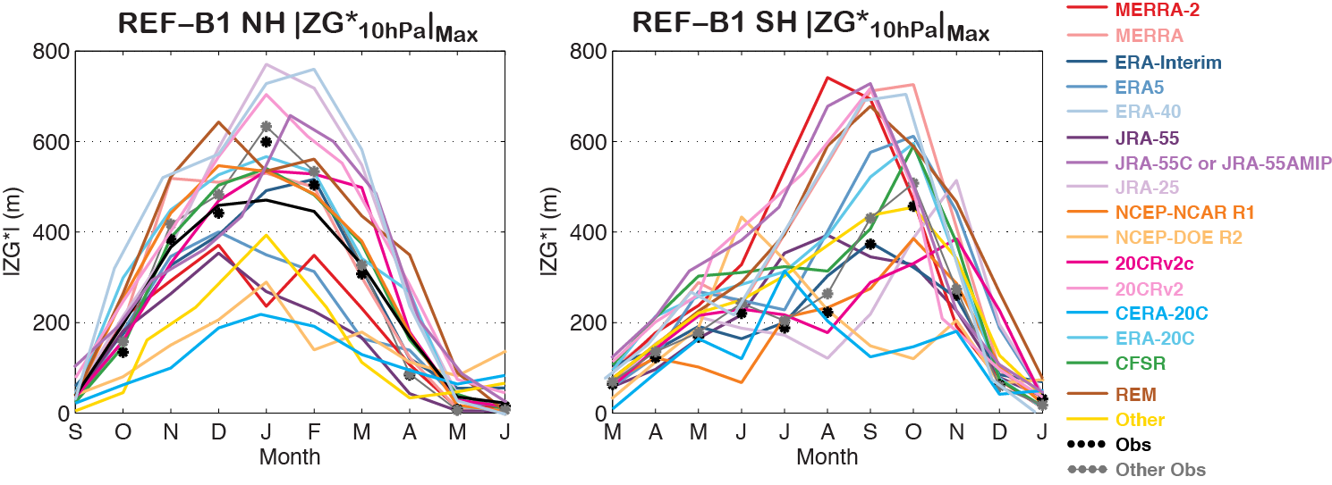
Suggested Colors for Intercomparing Reanalysis Timeseries from S-RIP:

The Sparc Reanalysis Intercomparison Project (S-RIP --> https://s-rip.github.io/) has a suggested list of colors to use for comparing reanalysis time-series. The list can be viewed here https://s-rip.ees.hokudai.ac.jp/mediawiki/index.php/Notes_for_Authors --> https://s-rip.github.io/report/colourdefinition.html The colors are available in CVS format below, in NCL, and in XLS. The link to the S-RIP page has examples for Python and IDL --> https://s-rip.github.io/report/colourtables.html.

Note that the URLs have changed. 

The colors are available in CVS format below, in NCL, and in XLS. 

CSV:

r,g,b,c,m,y,k,RGB Hexadecimal,reanalysis

226, 31, 38,  0,86.28,83.19,11.37,  E21F26,  MERRA-2

246, 153, 153,  0,37.8,37.8,3.53,  F69999,  MERRA

41, 95, 138,  70.29,31.16,0,45.88,  295F8A,  ERA-Interim

95, 152, 198,  52.02,23.23,0,22.35,  5F98C6,  ERA5

175, 203, 227,  22.91,10.57,0,10.98,  AFCBE3,  ERA-40

114, 59, 122,  6.56,51.64,0,52.16,  723B7A,  JRA-55

173, 113, 181,  4.42,37.57,0,29.02,  AD71B5,  JRA-55C or JRA-55 AMIP

214, 184, 218,  1.83,15.6,0,14.51,  D6B8DA,  JRA-25

245, 126, 32,  0,48.57,86.94,3.92,  F57E20,  NCEP-R1

253, 191, 110,  0,24.51,56.52,0.78,  FDBF6E,  NCEP-R2

236, 0, 140,  0,100,40.68,7.45,  EC008C,  20CRv2c

247, 153, 209,  0,38.06,15.38,3.14,  F799D1,  20CRv2

0, 174, 239,  100,27.2,0,6.27,  00AEEF,  CERA-20C

96, 200, 232,  58.62,13.79,0,9.02,  60C8E8,  ERA-20C

52, 160, 72,  67.5,0,55,37.25,  34A048,  CFSR

179, 91, 40,  0,49.16,77.65,29.8,  B35B28,  REM

255,215,0,  0,15.69,100,0,  FFD700,  Other

0, 0, 0,  0,0,0,100,  000000,  Obs

119, 119, 119,  0,0,0,53.33,  777777,  Other Obs

This image shows how the colors can be used.

Suggested Practices: Climatologies:

Use 1981-2010.

GOAT (Geophysical Observation Analysis Tool)

Analysis:

GOAT archives all geophysical data in a consistent format, thereby reducing the need to bother with the esoteric details of the particular datasets.

GOAT icludes a GUI based interface for intuitive browsing, subsetting and display of data in all spatial and temporal projections.

The GUI also provides some advanced analysis features such as:

• Calculation of climatology and anomalies
• Spatial and temporal filters
• Display differences between two fields
• Display superposition of two fields
• Include topography in display or analysis   
• Code generation (similar to the 'Generate Code' option in MATLAB figures)

Data retrieval:

GOAT intgrates with OPeNDAP sources and NetCDF files via a process referred to as 'linking' (GOAT LINK Format). GOAT also integrates with *.mat file archived in a GOAT standard format (GOAT MAT Format). The GOAT GUI also enables converting linked OPeNDAP and NetCDF archives to MAT Format. Information on GOAT archiving formats can be found in the GOAT documentation. 

OPeNDAP sources (GOAT LINK Format):

LINK archives do not require much disk space (typically a few MB per archive). A full list of available OPeNDAP LINK archive can be found here. Examples of available OPeNDAP LINK archives are

• MERRA (entire archive)
• 20th Century Reanalysis (entire archive)
• NCEP I and II (entire archives)
• ERA-40 (partial archive)
• ERA-Interim (entire archive. Uses a specially designed perl based protocol for communicating with the MARS server)
• ORA-S4 ocean reanalysis. 

NetCDF files (GOAT LINK Format):

GOAT indludes functions for automatically linking NetCDF files following the CMIP5 standard. In particular, the GOAT_CMIP5_LINK function (which can also be launched from the GOAT GUI) automatically finds all CMIP5 files in a specified folder and creates LINK archives for these files.

This functionality can be further extended to other datasets as a growing number of observational datasets are now available in CMIP5 archiving standard via the obs4MIPs and ana4MIPs projects.

Conversion of datasets to *.mat files (GOAT MAT Format)

GOAT includes a GUI based data download tool for automatically downloading and converting datasets to GOAT MAT Format (*.mat files).

Information on available datasets for download can be found here. 

The following datasets are available via the GUI based tool:

Atmosphere

• NCEP I and NCEP II
• 20th Century Reanalysis
• MERRA Daily

Clouds

• CloudsatCalipso (a combination of Cloudsat and Calipso by Jennifer. E. Kay)

Surface

• GISTEMP
• TRMM Daily
• ERSST (V3b)

Ocean:

• GODAS
• ECMWF ORA-S4
• World Ocean Atlas 2013

Lübken, F.-J., U. Berger, and G. Baumgarten (2013),

Temperature trends in the midlatitude summer mesosphere,

J. Geophys. Res. Atmos., 118, doi: 10.1002/2013JD020576.

A trend analysis of long term runs have been performed with the LIMA model (0-150 km altitude) applying the NOAA-CIRES 20^th Century Reanalysis (V2) from 2009 back to 1871. LIMA adapts the Reanalysis data (u,v,T) with global coverage every 6 hour below about 25 km applying a nudging method. Variations of green house gases CO₂ and O₃ have been predescribed according to observations. Trends have been estimated in the troposphere, stratosphere, and mesosphere at mid-latitudes for summer conditions (June - August).

As a main result trends are non-uniform with time.

Since the late 19th century, temperatures in the mesosphere have dropped by up to 5-7 K (10-12 K) on pressure (geometric) altitudes.

This is much more than typical trends in the troposphere and stratosphere. The summer mesosphere therefore reacts much more sensitive to climate change compared to lower altitudes.

Short summary:

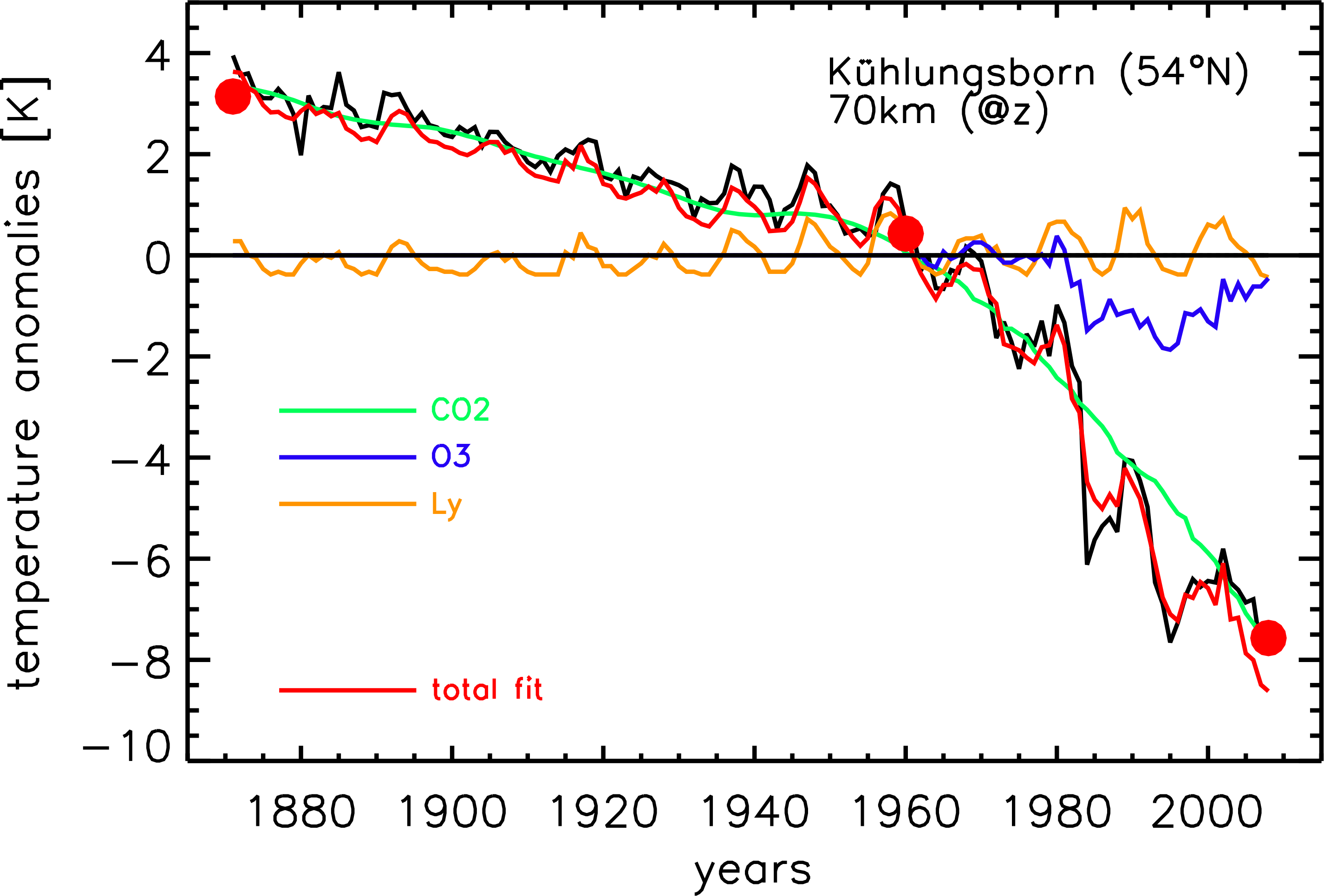
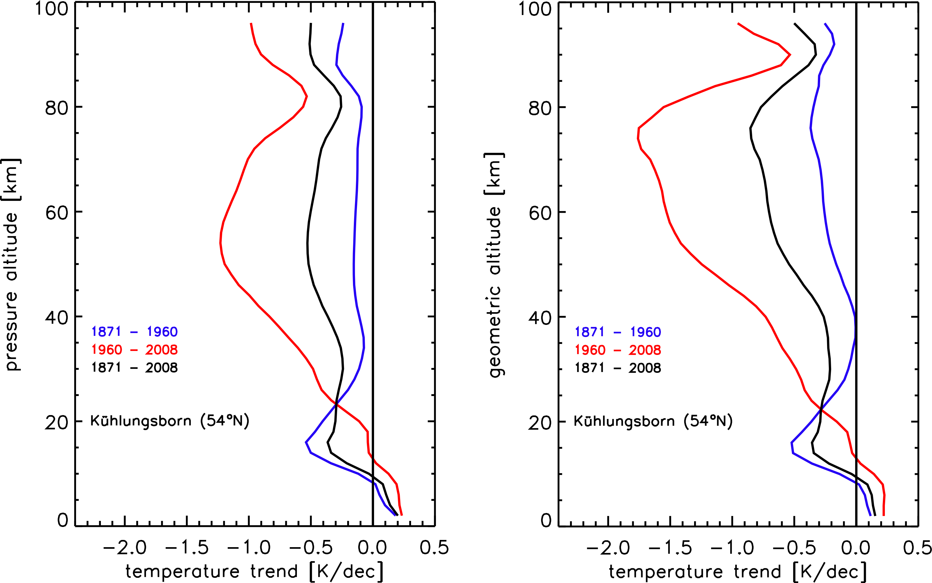
In Fig. 1 we show mean June to August temperatures at 54°N from LIMA at geometric height of 70 km based on NOAA-CIRES 20^th Century Reanalysis. We have performed a multivariate fit based on three functions (also shown in Fig. 1), namely CO₂(t), O₃(t), and Ly-alpha(t). The largest contribution to the long term temperature trend comes from CO₂, whereas O₃ has an impact in the last 30 years only (by construction), and Ly-alpha(t) causes a quasi-periodical modulation. Obviously, temperature trends are not uniform in time but accelerate since approximately the 1960s. Comparison with CO₂(t) clearly shows that this acceleration is due to an increase of carbon dioxide. We have calculated temperature trends in three periods, namely from the beginning of the time series (1871) to 1960, from 1960 to present time (2008), and over the entire period. The results are shown in Fig. 2. As expected, trends are larger in the second period. In pressure coordinates, total temperature trends are largest in the upper stratosphere and mesosphere, more precisely at 40-70 km. Trends are minimal around the mesopause. In geometric heights, trends are generally larger and, for the second period 1960-2008, clearly maximize in the mesosphere, where trends can be as large as -1.8 K/dec. We note that this trend analysis produces very similar results in comparison with a detailed trend analysis using ECMWF reanalysis data in the period 1961-2009 (for more details, see Lübken et al, JGR, 2013).

Fig.1: Temperature anomalies (=deviations from the June-August 1871-2009 mean) at z_geo=70 km at 54°N (Kühlungsborn, Germany) from 1871 to 2008 (black line). The result of a multivariate fit (red) consisting of CO₂(t) (green), O₃(t) (blue), and Ly-alpha(t) (orange) is also shown. Temperatures are marked at the beginning and at the end of the time series, and around 1960 where the trend changes markedly (red dots).

Fig.2: Temperature trends (June-August) for the location of Kühlungsborn 54°N) as a function of pressure (left) and geometric (right) altitudes. Black lines show the trend over the entire period (1871-2008), whereas blue and red lines show trends in the subperiods 1871-1960 and 1960-2008, respectively.

I suspect that the 20CR.v2 ensemble mean wind speeds provided publicly were calculated incorrectly, and I will briefly explain.

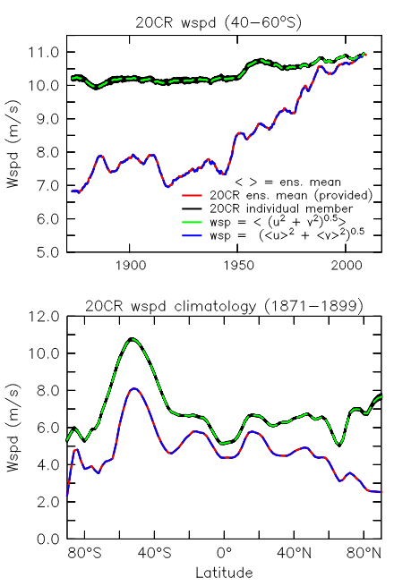
As confirmed in the attached plots, the ensemble mean speeds provided for 20CR were computed as:

wspd = [<u>^2 +<v>^2]^0.5



where <> indicates the ensemble mean. The correct calculation would be



wspd = < [u² + v²]^0.5 >



As you can see in the attached, the provided ensemble mean speeds look nothing like the speeds in the individual ensemble members, and appear  wrong.

After downloading all the individual ensemble members and recalculating the speeds using the correct formula above, I get an ensemble mean which is perfectly

consistent with the individual members (i.e. falls in the middle of them), as would be expected.

The ensemble mean wind speeds provided also look physically unrealistic (e.g. too low at extratropical latitudes prior to the 1990's), and exhibit unrealistically

large trends. When using the individual ensemble members, or the correctly re-calculated ensemble mean speed, these issues are corrected.

I suspect many users could be affected by this, and I hope that this info might be useful.

-Neil Swart

Note in the time-series plot attached the data are all smoothed with a 5-year wide boxcar. 

Truchelut, R., R. Hart, and B. Luthman, 2013: Global identification of previously undetected pre-satellite era tropical cyclone candidates in NOAA/CIRES 20th Century Reanalysis data. J. Appl. Meteor. Climatol. doi:10.1175/JAMC-D-12-0276.1.

For full documentation and results of the project, please visit: http://moe.met.fsu.edu/tcce/

Project Abstract

Prior to the satellite era, limited synoptic observation networks led to an indefinite number of tropical cyclones (TCs) remaining undetected. This period of decreased confidence in the TC climatological record includes the first two-thirds of the 20th Century. While prior studies found this undersampling exists, disagreement regarding its magnitude has caused difficulties in interpreting multi-decadal changes in TC activity.



Previous research also demonstrated that reanalyses can be used to extend TC climatology, utilizing the NOAA/CIRES 20th Century Reanalysis to manually identify previously unknown Atlantic Basin potential TCs. The results significantly expand upon the scope of the earlier work, using a filtering algorithm to identify TC candidate events in all tropical basins for the years 1871-1979. The result is the first quantitative and objective global TC candidate event counts for the decades prior to formal recordkeeping.



Verification using ship reports and other in situ observations performed on a subset of the events indicates that the algorithm identifies potential missing TCs at a success rate of 25%-50%, depending on the basin. As our team has performed the verification process on only a small fraction of the thousands of candidate events identified, maps have been made publically available containing model and observational data produced at 6 hour intervals for each candidate event. These images, as well as full documentation of our research procedures, is provided at the links above. It is our hope that ongoing and future TC climatology revision efforts will use this data as a source of independent guidance in order to produce a more complete record of historical tropical cyclone activity.

We hope you find our work useful, and please do not hesitate to contact us directly with questions or specific data requests.

Ryan Truchelut (ret08@fsu.edu) and Robert Hart (rhart@fsu.edu)

Florida State University Meteorology

From Chung, E.-S., B. J. Soden, B. J. Sohn, and J. Schmetz (2013), An assessment of the diurnal variation of upper tropospheric humidity in reanalysis data sets, J. Geophys. Res. Atmos., 118, doi:10.1002/jgrd.50345.

Diurnal variations of upper tropospheric humidity in five different reanalysis datasets are compared over convective land and ocean regions, and evaluated using multiple satellite observations as a reference. All reanalysis datasets reproduce the day/night contrast of upper tropospheric humidity and the land/ocean contrast in the diurnal amplitude. The infrared satellite measurements indicate a slightly later diurnal minimum over land relative to most reanalyses and the microwave satellite measurements, suggesting that cloud masking of the infrared radiances may introduce a small (~ 3 hr) bias in the phase. One reanalysis exhibits a substantially different diurnal cycle over land which is inconsistent with both infrared and microwave satellite measurements and other reanalysis products. This product also exhibits a different covariance between vertical velocity, cloud water and humidity than other reanalyses, suggesting that the phase bias is related to deficiencies in the parameterization of moist convective processes.

Diurnal anomaly of Meteosat-5 water vapor channel brightness temperature simulated from NCEP/DOE, 20th Century Reanalysis, ERA-40, ERA-Interim, and MERRA over the convectively active regions of Africa and the Atlantic Ocean for the period 1984-2004. The red lines denote the diurnal anomaly of observed brightness temperature for the same period.

Citation: L'Heureux, M.L., S. Lee, and B. Lyon, 2013: Recent multidecadal strengthening of the Walker circulation across the tropical Pacific. Nature Clim Change, doi: 10.1038/nclimate1840.

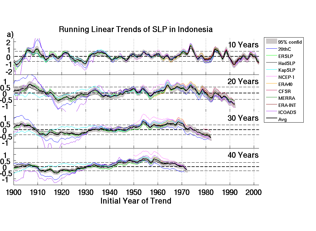
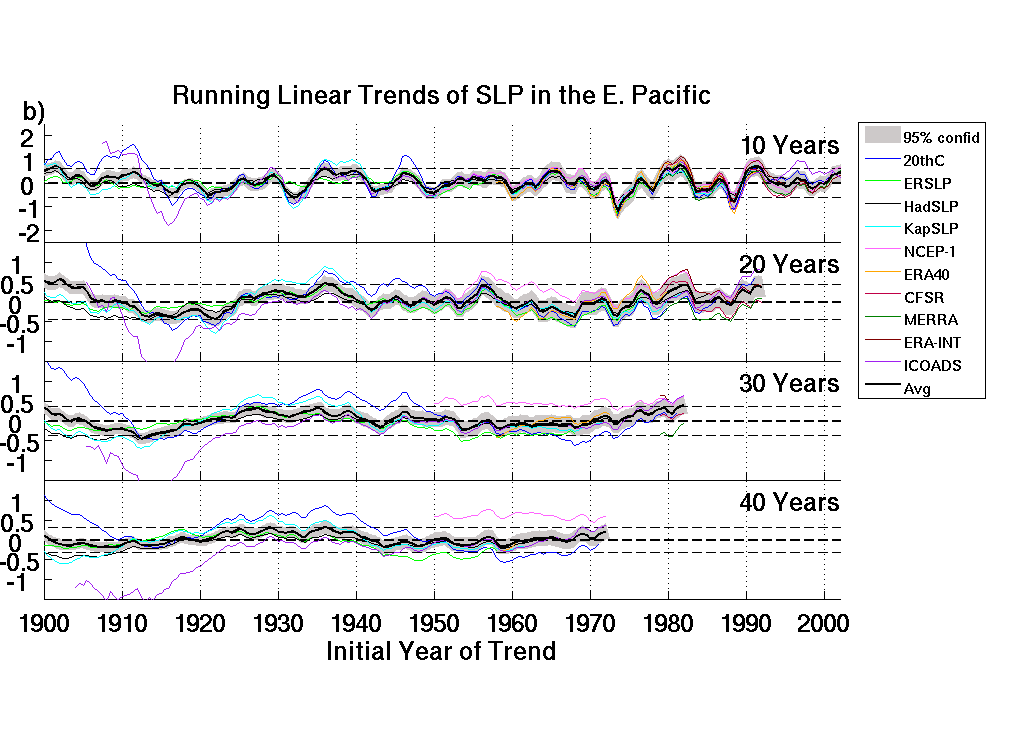
Ten different datasets from reanalyses, reconstructions, and in situ measurements are examined for sea level pressure (SLP) trends over the tropical Pacific.  Instead of fitting a single least squares linear trend through the entire 1900-2011 record, running linear trends are calculated every six months over varying length windows (10-, 20-, 30-, and 40-year).  For the 20-40 year windows over Indonesia (110-160E, 10S-10N), a gradual increase from negative to positive SLP trends is evident beginning in 1910-1920 (see top figure below).  Then, starting in 1955-1965, the the positive trends cease growing and eventually trends become significantly negative over the last several decades. In contrast, over the Eastern Pacific (130-80W, 10S-10N), trends are less significant but there is evidence for a tendency towards positive SLP trends starting in the late 1950s or 1960s (see bottom figure below).  The tendency towards lower SLP over Indonesia and higher SLP over the eastern Pacific suggests a strengthening Walker circulation over the last half of the 20^th century.  This increase in the Walker circulation becomes even more apparent when ENSO variability (using the Nino-3.4 index) is linearly removed from the datasets.  Moreover, the tendency for a strengthening Walker circulation appears to be nearly concurrent with the shift toward positive trends in global average temperatures.

While not shown below (see supplementary info), we note that a significant lack of in situ SLP data (ICOADS.v2.5) over the tropical Pacific is linked to larger disagreement in the datasets during the first half of the 20th century. Therefore, caution is recommended when interpreting the observed linear SLP trends prior to the 1950s.   

All the best reanalyses include uncertainty estimates, and I've been using fog to mark times and regions where the analyses are too uncertain to provide much value. This works well with 20CR - it's easy to make a compelling plot showing a relatively low spread in regions with lots of observations, and a much wider spread elsewhere.

But there are many different possible metrics for uncertainty: I originally chose the ratio of ensemble standard deviation (esd) to climatological standard deviation (csd), and this mostly works, but it undervalues the reanalysis in places where there is a lot of weather. If a big storm is coming but the magnitude and location are uncertain, esd can be very large, but the reanalysis is still informative. So I should include signal magnitude as well as spread.

The obvious approach is some combination of csd/esd and (em-cm)/csd (em=ensemble mean). Gil pointed me at the concept of Relative Entropy - more impressively known as Kullback-Leibler divergence. The K-L divergence between the reanalysis ensemble and the climatological distribution (Dkl(R||C)) is the information lost when using the climatology as an estimator of the reanalysis. In general it's hard to calculate, but under a reasonable set of simplifying assumptions:

Dkl(R||C) = 1/2*(ln(csd**2/esd**2) + (esd**2/csd**2)-1 + (em-cm)**2/csd**2)

(That's for a single variable - I'm only using MSLP here. It does generalise to multiple variables (could add temperature, precip etc.), but results are dominated by the variable where 20CR has most skill, so just using MSLP is reasonable).

So where the analysis is unconstrained by observations, esd=csd and em=cm and Dkl(R||C)=0 (might as well use the climatology). As we add observational constraints either esd will shrink or em will become different from cm or both, and Dkl(R||C) becomes positive.

This would be fine if the reanalysis were based on a perfect model, but in reality, in the absence of observational constraints esd!=csd and em!=cm and Dkl(R||C) is large. I wangle round this by replacing climatology with a, somewhat arbitrary, Uninformed distribution (U) and choose usd=max(esd,csd) and um=30-year running mean from reanalysis. Dkl(R||U) is then 0 where the reanalysis is unconstrained and increases with observational constraints.

The results look like this (plots show prmsl and 10m wind actuals, and air.2m anomalies - yellow dots mark observations):

For 1987:

and for 1918:

I do still have to choose an arbitrary threshold for fog (here Dkl(R||U) <=1) but it doesn't make an enormous difference as Dkl(R||U) goes from zero to big quite abruptly.  I'd like to make such a video for the entire 140-year span of 20CR, to show the fog dissipating as the observations coverage increased, but it would take forever to render and hours even to watch. But the method is general - it should work at any timescale - so I've made the long video using monthly data:

Monthly weather is a bit random and discontinuous, but it does show the improvement in 20CR as the observations coverage increases. I like the variable but persistent effect of the Port Stanley observation in the Falklands.

It still feels a bit wrong to me: I was originally working just with the ensemble spread, and Dkl is exponentially more sensitive to the mean anomaly than to the spread - so the weather matters much more than the analysis precision. But the literature seems clear that it's the right metric.

Brönnimann, S., O. Martius, H. von Waldow, C. Welker, J. Luterbacher, G.P. Compo, P.D. Sardeshmukh, and T. Usbeck, 2012:Extreme winds at northern mid-latitudes since 1871. Meteorol. Zeit., 21, 13-27, doi: 10.1127/0941-2948/2012/0337.

Studying a sufficiently large sample of extremes or analysing the statistics of their occurrence, including trends, is hampered by the length of the existing observation-based record. New data sets such as the Twentieth Century Reanalysis (20CR), which consists of an ensemble of 56 members, significantly extend our record back in time. In this paper, we present examples of extremes of winds at northern hemisphere mid-latitudes in 20CR to illustrate challenges and opportunities for analysing extremes over a longer period than previously possible. For four representative storms from Europe and North America, 20CR provides a relatively good depiction of the synoptic-scale meteorological development, although it misses smaller scale features as well as local effects due to orography. For analysing trends of extreme winds, it is shown that the individual ensemble members should be used, rather than the ensemble mean, which appears to be biased towards lower wind speeds early in the record. For the studied locations, decadal variability and trends can best be characterised after around 1950, when the ensemble variance remains consistent. Different methodological approaches for studying changes in extreme winds are discussed. Finally, we show hemispheric maps of trends in extreme wind speeds since 1950.

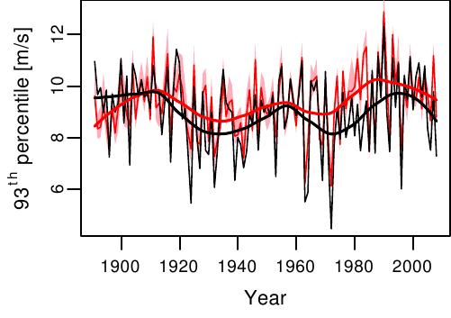
The seasonal (Oct-Mar) 93rd percentile of daily wind maxima from hourly observations from Zurich (black), from the 20CR ensemble mean 0.995 sigma level wind at the nearest grid point (red) and for the corresponding range from the ensemble members. The thick lines are smoothed with a spline function.

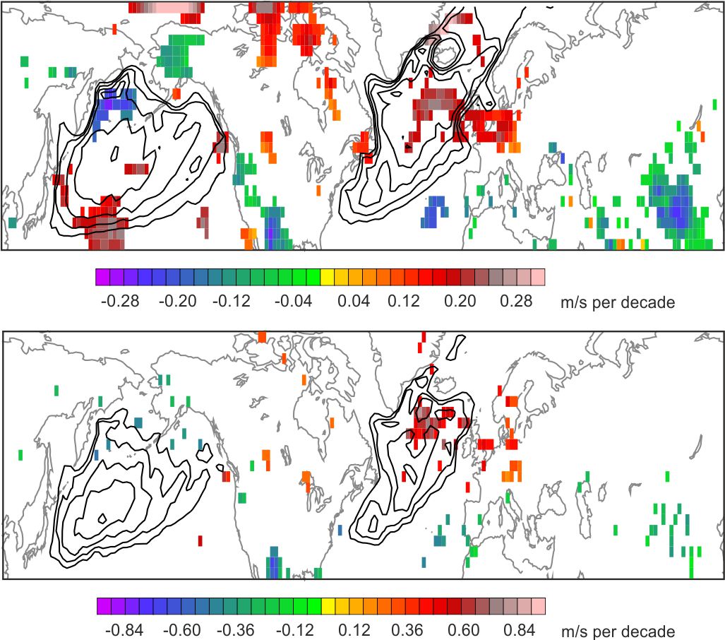
Map of the trend in the annual 98th percentile (top) and annual maximum (bottom) 0.995 sigma level wind  from 20CR for the period 1950-2008. Shown is the mean of the trend from the individual members, but only if 90% of the ensemble members exhibit a significant (p<0.05) trend. Contours denote the ensemble average of the 98th percentile and annual maximum 0.995 sigma level wind, respectively, with contours starting at 20 m/s (top) and 30 m/s (bottom) and an interval of 1 m/s.