Both observational and numerical studies suggest that fall snow cover extent over Eurasia is linked to subsequent winter variations in the predominant Northern Hemisphere teleconnection pattern, known as the Arctic Oscillation (AO). The present study uses the recent 20CR reanalysis to explore the snow-AO relationship over the entire 20th century for the first time. 20CR is first shown to have a consistently realistic simulation of the onset of the Eurasian snow cover compared to a large number of in-situ observations. It is then used to explore the snow-AO relationship over both the satellite and pre-satellite periods. Results show that this teleconnection is not stationary and did not emerge until the 1970's. The possible modulation of the teleconnection by the Quasi-Biennal Oscillation (QBO) is then discussed, as it could have favored the influence of snow anomalies on the Arctic Oscillation in recent decades. These results have important implications for seasonal forecasting and suggest, in particular, that statistical predictions of the wintertime AO should not be based on snow predictors alone.

 

Reference : Peings Y., E. Brun, V. Mauvais, H. Douville (2013) How stationary is the relationship between Siberian snow and Arctic Oscillation over the 20th century ? Geophysical Research Letters, DOI: 10.1029/2012GL054083.

 

 

Figure 1. 20CR snow detection performance: percentage of October days with snow/no snow in both 20CR snow cover and HSDSD data (threshold 5cm) over 1881-1994. b) Difference in % between the 20CR and NSIDC snow detection performance over 1972-1994. c) Observed snow frequency in % of October days over 1972-1994, defined as the ratio of HSDSD data higher than 5 cm.

 

Figure 2. Timeseries and correlations for the following indices: AO-CPC ; SAI-NSIDC ; SAI-20CR from weekly data over the 1973/74-2006/2007 period. Stars indicate the significance of correlations : ** p<0.01 ; * p<0.05. b) Correlations on a 21-year moving window: AO-CPC vs SAI-20CR; AO-20CR vs SAI-20CR; AO-CPC vs SAI NSIDC; AO-CPC vs SCI-20CR; AO-20CR vs SCI-20CR ;AO-CPC vs SCI NSIDC. The 95% confidence level for correlations is indicated by the horizontal dashed lines. SAI-20CR is computed from daily data

 

 

The reanalysis provides us with simultanious estimates of many different variables; so we can make rich reconstructions of particular events, if we can work out how to plot several variables simultaniously. For Snows of Yesteryear, we wanted a visualisation of the UK winter of 1962/3, possibly the coldest in the twentieth century in England and Wales, to provide context and contrast for the documentary accounts of weather impact being collected by the project.

This video shows sea-level pressure (black contours), 10m wind speed and direction (arrows), and 2m temperature anomaly (arrow colours), from the 20th Century reanalysis. The uncertainties for this time and place are small, so we can have confidence in the circulation reconstructions, and we do indeed see the southern UK being dominated by cold easterlies, particularly in January (the coldest month).

 

To include a video in a page on reanalysis.org:

1. Put the video up on Vimeo
2. Click the 'share' icon in the video top right on it's vimeo page (the paper plane - see the video above).
3. Copy the 'embed' code (text starting '<iframe ').
4. Edit the reanalysis.org page using the plain text editor.
5. Paste the copied embed code into the page text at the selected point.

something similar can surely be done with YouTube instead of Vimeo, but I haven't tried.

 

Lavers, D.A., G. Villarini, R.P. Allan, E.F. Wood, and A.J. Wade, The detection of atmospheric rivers in atmospheric reanalyses and their links to British winter floods and the large-scale climatic circulation, Journal of Geophysical Research, 117, D20106, doi:10.1029/2012JD018027, 2012.

 

Atmospheric rivers (ARs) are narrow bands of enhanced water vapor transport in the lower troposphere, and are the cause of extreme precipitation and floods over mid-latitude regions.  This study introduces an algorithm (based on the vertically-integrated horizontal Water Vapor Transport, IVT) for the detection of persistent ARs (lasting 18 hours or longer) in five atmospheric reanalysis products.  The reanalyses considered were: (1) NCEP Climate Forecast System (CFSR), (2) ECMWF ERA-Interim (ERAIN), (3) Twentieth Century Reanalysis (20CR), (4) NASA Modern Era Retrospective-Analysis for Research and Applications (MERRA), and (5) NCEP–NCAR.

Figure 1: Time series of the number of persistent ARs in each winter half-year (October to March) over 1980–2010 in the five reanalyses (left y-axis).  The black dashed line represents the winter half-year Scandinavian Pattern index (anomaly values shown on the right y-axis).  The total number of ARs for each reanalysis product is given in the legend.

Time series of the number of detected ARs in each winter half-year over 1980–2010 in the five reanalyses are shown in Figure 1 (taken from JGR paper).  The number of ARs varies between about 2 and 14 events per winter.  Each product identifies a different number of ARs ranging from 190 in CFSR to 264 in 20CR, which may be partly caused by the different IVT threshold values used for each reanalysis, as well as the different assimilating models and data used. As shown in Figure 1, a negative dependence was found between AR frequency and the winter half-year Scandinavian Pattern. In conclusion, the generally good agreement of AR occurrence between the reanalyses suggests that realistic sea surface temperatures and atmospheric circulation, used in the five products, are sufficient for simulating the AR structures.

 

Figure 2: The IVT (in kg m^-1 s^-1) for (a) 20CR, (c) CFSR, (d) ERAIN, (e) MERRA, (f) NCEP–NCAR and (b) 20CR MSLP field (in hPa) at 1200 UTC 10^th December 1994 before the largest flood event on 11^th December 1994 in the Ayr at Mainholm basin in Scotland.  The “L” and “H” in panel (b) refer to the Low and High pressure centres respectively; the black dots in the panels mark the location of the Ayr at Mainholm basin.

An example of an AR captured in the five reanalyses is shown in Figure 2 (taken from JGR paper); this AR was behind the largest flood in one of the study river basins. The effect of the different reanalysis grid resolutions is shown, with the peak IVT and hence AR region (as shown by the red and orange colors) in the finer resolution CFSR, ERAIN and MERRA products occupying a smaller region than in the 20CR or NCEP-NCAR. 

A strong link exists between the detected ARs and the biggest winter floods in the nine study basins. In one western British basin about 80% of the 31 largest floods followed a persistent AR. As the largest floods in these basins occur in the winter, these results provide evidence that ARs control a large part of the upper tail of the flood peak distribution.   

 

 

Wang, J., W. Wang, X. Fu, K.-H. Seo, 2012: Tropical intraseasonal rainfall variability in the CFSR. Climate Dynamics, 38, 2191-2207, http://link.springer.com/article/10.1007/s00382-011-1087-0

While large-scale circulation fields from atmospheric reanalyses have been widely used to study the tropical intraseasonal variability, rainfall variations from the reanalyses are less focused. Because of the sparseness of in situ observations available in the tropics and strong coupling between convection and large-scale circulation, the accuracy of tropical rainfall from the reanalyses not only measures the quality of reanalysis rainfall but is also to some extent indicative of the accuracy of the circulations fields. This study analyzes tropical intraseasonal rainfall variability in the recently completed NCEP Climate Forecast System Reanalysis (CFSR) and its comparison with the widely used NCEP/NCAR reanalysis (R1) and NCEP/DOE reanalysis (R2). The R1 produces too weak rainfall variability while the R2 generates too strong westward propagation. Compared with the R1 and R2, the CFSR produces greatly improved tropical intraseasonal rainfall variability with the dominance of eastward propagation and more realistic amplitude. An analysis of the relationship between rainfall and large-scale fields using composites based on Madden-Julian Oscillation (MJO) events shows that, in all three NCEP reanalyses, the moisture convergence leading the rainfall maximum is near the surface in the western Pacific but is above 925 hPa in the eastern Indian Ocean. However, the CFSR produces the strongest large-scale convergence and the rainfall from CFSR lags the column integrated precipitable water by 1 or 2 days while R1 and R2 rainfall tends to lead the respective precipitable water. Diabatic heating related to the MJO variability in the CFSR is analyzed and compared with that derived from large-scale fields. It is found that the amplitude of CFSR-produced total heating anomalies is smaller than that of the derived. Rainfall variability from the other two recently produced reanalyses, the ECMWF Re-Analysis Interim (ERAI), and the Modern Era Retrospective-analysis for Research and Applications (MERRA), is also analyzed. It is shown that both the ERAI and MERRA generate stronger rainfall spectra than the R1 and more realistic dominance of eastward propagating variance than R2. The intraseasonal variability in the MERRA is stronger than that in the ERAI but weaker than that in the CFSR and CMORPH.

Wavenumber-frequency spectra of 10ºS–10ºN average of raw daily–mean anomalies of precipitation. a CMORPH; b R1; c R2; and d CFSR The unit is 0.001 mm² days⁻². Contours are shaded starting at 6 with an interval of 3.

Wavenumber-frequency spectra of 10ºS–10ºN average of raw daily–mean anomalies of precipitation. a ERAI; and b MERRA. 

 

Wang, W., P. Xie, S.-H. Yoo, Y. Xue, A. Kumar and X. Wu, 2011:  An assessment of the surface climate in the NCEP climate forecast system reanalysis. Climate Dynamics, 37, 1601-1620

http://link.springer.com/article/10.1007%2Fs00382-010-0935-7

This paper analyzes surface climate variability in the climate forecast system reanalysis (CFSR) recently completed at the National Centers for Environmental Prediction (NCEP). The CFSR represents a new generation of reanalysis effort with first guess from a coupled atmosphere–ocean–sea ice–land forecast system. This study focuses on the analysis of climate variability for a set of surface variables including precipitation, surface air 2-m temperature (T2m), and surface heat fluxes. None of these quantities are assimilated directly and thus an assessment of their variability provides an independent measure of the accuracy. The CFSR is compared with observational estimates and three previous reanalyses (the NCEP/NCAR reanalysis or R1, the NCEP/DOE reanalysis or R2, and the ERA40 produced by the European Centre for Medium-Range Weather Forecasts). The CFSR has improved time-mean precipitation distribution over various regions compared to the three previous reanalyses, leading to a better representation of freshwater flux (evaporation minus precipitation). For interannual variability, the CFSR shows improved precipitation correlation with observations over the Indian Ocean, Maritime Continent, and western Pacific. The T2m of the CFSR is superior to R1 and R2 with more realistic interannual variability and long-term trend. On the other hand, the CFSR overestimates downward solar radiation flux over the tropical Western Hemisphere warm pool, consistent with a negative cloudiness bias and a positive sea surface temperature bias. Meanwhile, the evaporative latent heat flux in CFSR appears to be larger than other observational estimates over most of the globe. A few deficiencies in the long-term variations are identified in the CFSR. Firstly, dramatic changes are found around 1998–2001 in the global average of a number of variables, possibly related to the changes in the assimilated satellite observations. Secondly, the use of multiple streams for the CFSR induces spurious jumps in soil moisture between adjacent streams. Thirdly, there is an inconsistency in long-term sea ice extent variations over the Arctic regions between the CFSR and other observations with the CFSR showing smaller sea ice extent before 1997 and larger extent starting in 1997. These deficiencies may have impacts on the application of the CFSR for climate diagnoses and predictions. Relationships between surface heat fluxes and SST tendency and between SST and precipitation are analyzed and compared with observational estimates and other reanalyses. Global mean fields of surface heat and water fluxes together with radiation fluxes at the top of the atmosphere are documented and presented over the entire globe, and for the ocean and land separately.

Precipitation climatology (contour) and differences (shading) from the observation taken as the average of CMAP and GPCP. a Observation, b R1, c R2, d ERA40, and e CFSR. Contours are plotted at 2, 4, 8, and 12 mm/day, and shadings are at −4, −2, −1, −0.5, 0.5, 1, 2, and 4 mm/day. Global mean (GM) climatology is shown above each panel

 

Ebisuzaki, W. and L. Zhang, 2011: Assessing the performance of the CFSR by an ensemble of analyses. Climate Dynamics, 37, 2541-2550

http://link.springer.com/article/10.1007/s00382-011-1074-5#

The Climate Forecast System Reanalysis (CFSR, Saha et al. in Bull Am Meteor Soc 91:1015–1057, 2010) is the latest global reanalysis from the National Centers of Environmental Prediction (NCEP). In this study, we compare the CFSR tropospheric analyses to two ensembles of analyses. The first ensemble consists of 12 h analyses from various operational analyses for the year 2007. This ensemble shows how well the CFSR analyses can capture the daily variability. The second ensemble consists of monthly means from the available reanalyses from the years 1979 to 2009 which is used to examine the trends. With the 2007 ensemble, we find that the CFSR captures the daily variability in 2007 better than the older reanalyses and is comparable to the operational analyses. With the ensemble of monthly means, the CFSR is often the outlier. The CFSR shows a strong warming trend in the tropics which is not seen in the observations or other reanalyses.

 

The 200 hPa height (m) for Singapore (grid cell average). The time series were low passed filtered by a 12 months running mean. Shown are CFSR (red), ERA-40 (orange), JRA-25 (light blue), MERRA (green), R1 (blue), R2 (black) and the observation (thick black line).

 

Kumar, A., L. Zhang and W. Wang, 2012: Sea Surface Temperature - Precipitation Relationship in Different Reanalyses. Monthly Weather Review, doi: http://dx.doi.org/10.1175/MWR-D-12-00214.1

The focus of this investigation is how the relationship at intraseasonal time scales between sea surface temperature (SST) and precipitation (SST-P) varies among different reanalyses. The motivation for this work was spurred by a recent report that documented that the SST-P relationship in Climate Forecast System Reanalysis (CFSR) was much closer to that in the observation than it was for the older generation of reanalysis – NCEP/NCAR reanalysis (R1) and NCEP/DOE reanalysis (R2). Further, the reason was attributed either to the fact that the CFSR is a partially coupled reanalysis, while R1 and R2 are atmospheric alone reanalyses, or that R1 and R2 use the observed weekly averaged SST.

The authors repeated the comparison of the SST-P relationship among R1, R2, and CFSR, as well as two recent generation of atmosphere alone reanalyses, the Modern Era-Retrospective-analysis for Research and Applications (MERRA) and the ECMWF Re-Analysis Interim (ERAI). The results clearly demonstrate that the differences in SST-P relationship at intraseasonal time scales across different reanalyses are not due to whether the reanalysis system is coupled or atmosphere alone, but are due to the specification of different SSTs. SST-P relationship in different reanalyses, when computed against a single SST for the benchmark, demonstrates a relationship that is common across all the reanalyses and observations.

Lead-lag SST-precipitation correlation for various reanalyses and for observations over the tropical western Pacific (averaged over 10°S–10°N, 130°–150°E) for respective SSTs were used (left panel), and for NCDC SST as the benchmark (right panel). Negative (positive) lag in days on the x axis indicates days by which the SST leads (lags) the precipitation.

Paek, H. and H.-P. Huang (2012), A comparison of the interannual variability in atmospheric angular momentum and length-of-day using multiple reanalysis data sets, J. Geophys. Res., 117, D20102, doi:10.1029/2012JD018105. 

This study performs an intercomparison of the interannual variability of atmospheric angular momentum (AAM) in eight reanalysis datasets for the post-1979 era.  The AAM data are further cross validated with the independent observation of length-of-day (LOD). The intercomparison reveals a close agreement among almost all reanalysis datasets, except that the AAM computed from the 20^th Century Reanalysis (20CR) has a noticeably lower correlation with LOD and with the AAM from other datasets.  This reduced correlation is related to the absence of coherent low-frequency variability, notably the Quasi-biennial Oscillation, in the stratospheric zonal wind in 20CR.  If the upper-level zonal wind in 20CR is replaced by its counterpart from a different reanalysis dataset, a higher value of the correlation is restored.  The correlation between the AAM and the Nino3.4 index of tropical Pacific SST is also computed for the reanalysis datasets. In this case, a close agreement is found among all, including 20CR, datasets. This indicates that the upward influence of SST on the tropospheric circulation is well captured by the data assimilation system of 20CR, which only explicitly incorporated the surface observations.  This study demonstrates the overall close agreement in the interannual variability of AAM among the reanalysis datasets.  This finding also reinforces the view expressed in a recent work by the authors that the most significant discrepancies among the reanalysis datasets are in the long-term mean and long-term trend. Paek and Huang 2012

   The time series of ∆LOD (red curve, converted to an equivalent ∆AAM using Eq. (3)) and ∆AAM (blue curve) from different reanalysis datasets: (a) NCEP R-1, (b) NCEP R-2, (c) CFSR, (d) 20CR, (e) ERA-40, (f) ERA-Interim, (g) JRA-25, and (h) MERRA. The time series of ∆Nino3.4 from HadISST is imposed as the green curve in panel (h). The units for ∆AAM and ∆Nino3.4 are 10²⁵ kg m² s^-1 and 1 °C, respectively. The time series for ∆AAM in panel (e) is slightly shorter due to the shorter record of the ERA-40 dataset.

   The time series of ∆M_R,STRAT for four selected reanalysis datasets including 20CR. (b) The original (dark blue) and the modified ∆AAM (light blue) for 20CR. The modified ∆AAM is calculated by replacing the zonal wind in the stratosphere by that from NCEP R-1. See text for detail.  The time series of ∆LOD (converted to an equivalent ∆AAM) is also shown as the red curve. The unit for ∆AAM is 10²⁵ kg m² s^-1.

 

Purpose: To perform basic extrapolations resulting in continuous fields of  NASA MERRA reanalyses for selected model levels where pressure values are greater than the surface pressure (i.e., filling in model grid points "below ground" with defined values). This could be useful where a continuous global field is needed, such as in modeling applications or spherical harmonic analyses. Code samples are included, below.  Geopotential heights are extrapolated by applying the hydrostatic equation and equation of state, as are temperature fields using adiabatic lapse rate approximations (moist or dry). 

Background reference from the MERRA FAQs (https://gmao.gsfc.nasa.gov/research/merra/faq.php)

Q. 6 "Why are there such large discrepancies at 1000MB and 850MB between MERRA and other Reanalyses?"

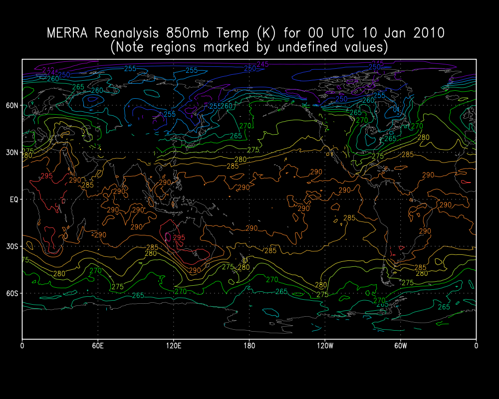
A. "The GEOS5 data assimilation system used to produce MERRA does not (or did not at the time of production) extrapolate data to pressure levels greater than the surface pressure. These grid points are marked by undefined values. The result is that area averages that include these points will not be representative compared to other data sets without additional screening. Time averages, such as monthly means, may also have substantial differences at the edges of topography. The lowest model level data and surface data are available so that users can produce their own extrapolation. A page discussing this issue is available. See http://gmao.gsfc.nasa.gov/research/merra/pressure_surface.php.   "

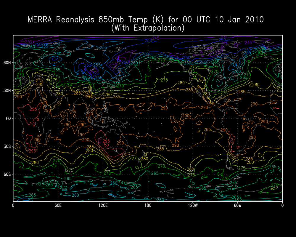
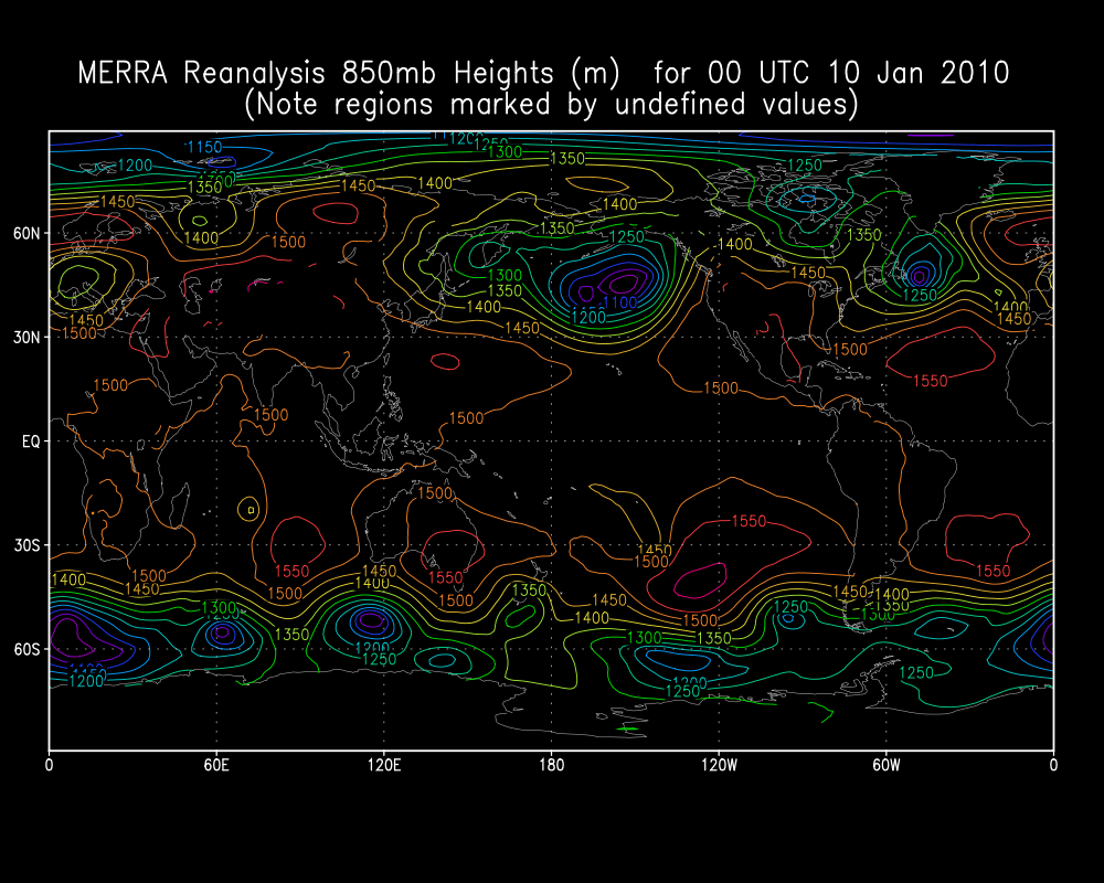
Below, note regions corresponding to high model topography where contours end due to undefined values in a sample MERRA Reanalysis plot (for example, portions of Rocky Mountains, Andes Mountains, Tibetan Plateau, Antarctica):

 

With extrapolation, the values are "filled in", as this figure shows (below):

 

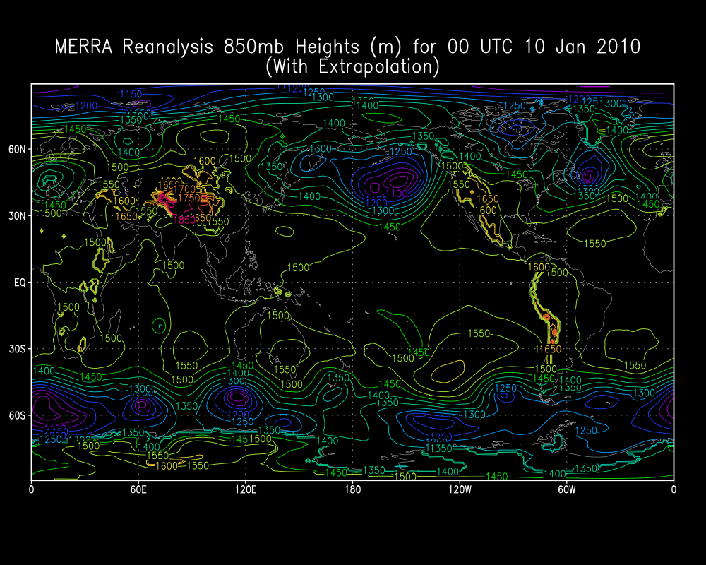
Here is another example with Geopotential height:

 

And, after extrapolation:

 

Below are sample codes and scripts that perform extrapolation on 5 variables from a MERRA NetCDF file.

Software needed: GrADS, Fortran compiler, Unix/Linux shell environment.

Need a MERRA NetCDF or HDF file along with the following:

1.Shell executable extrap.csh:   Runs programs, creates output.  Calls grads scripts and fortran executable

*********************************** 

*********************************************

 

2. Two GrADS control files are needed:

check_filled_9999.ctl (views output w/-9999 set as undefined):

 

'reinit'

'sdfopen MERRA300.prod.assim.inst3_3d_asm_Cp.20100110.SUB_1.nc'

'set x 1 288'

'set y 1 144'

'set gxout fwrite'

'set fwrite tot_merra_filled_9999.prs'

t=1

while (t <= 8)

 'set t 't

say 'Analysis time is 't

*height

  z=1

  while (z<=17)

    'set  z 'z

    'd const(maskout(h,h),-9999.,-u)'

    z=z+1

  endwhile

*

*Temperature

  z=1

  while (z<=17)

    'set  z 'z

    'd const(maskout(t,t),-9999.,-u)'

    z=z+1

  endwhile

*

*u-wind

  z=1

  while (z<=17)

    'set  z 'z

    'd const(maskout(u,u+1000),-9999.,-u)'

    z=z+1

  endwhile

*

*v-wind

  z=1

  while (z<=17)

    'set  z 'z

    'd const(maskout(v,v+1000),-9999.,-u)'

    z=z+1

  endwhile

*




*RH

  z=1

  while (z<=17)

    'set  z 'z

    'd const(maskout(rh,rh),-9999.,-u)'

    z=z+1

  endwhile

*

 t = t + 1

endwhile

'disable fwrite'

'quit'

 

 

 

 4.  Fortran file extrap_merra.f:

 Code to perform extrapolation, called in extrap.csh.




 

 

 

 

 

Contact: Lee Byerle 

Zhang, Q., H. Körnich and K. Holmgren, 2012: How well do reanalyses represent the southern African precipitation? Clim. Dyn., DOI: 10.1007/s00382-012-1423-z.

http://dx.doi.org/10.1007/s00382-012-1423-z

Monthly-mean precipitation observations over southern Africa are used to evaluate the performance of eight global reanalyses: ERA-40, ERA-interim, JRA-25, MERRA, CFSR, NCEP-R1, NCEP-R2 and 20CRv2. All eight reanalyses reproduce the regionally averaged seasonal cycle fairly well; a few spatial mismatches with the observations are found in the climate mean for the rainy season. Principal component analyses show a dipole in the leading modes of all reanalyses, however with crucial differences in its spatial position.

Possible reasons for the differences between the reanalyses are discussed on the basis of the ERA-interim and 20CRv2 results. A comparison between the moisture transports shows that ERA-interim manifests a very strong moisture convergence over the eastern equatorial Atlantic, resulting in the strong precipitation here. This excessive convergence may be due to the water–vapor assimilation and convection parameterization. Over the Indian Ocean, the ITCZ is shifted northward in ERA-interim compared to its position in 20CRv2. This discrepancy is most likely attributable to the meridional SST gradients in the Indian Ocean which are significantly larger in the ERA-interim than those in the 20CRv2, and the resulting atmospheric response prevents a southward shift of the ITCZ.

Overall, the consistent description of the dynamical circulation of the atmosphere and the hydrological cycle appears as a crucial benchmark for reanalysis data. Based on our evaluation, the preferential reanalysis for investigating the climate variability over southern Africa is 20CRv2 that furthermore spans the longest time period, hence permitting the most precise investigations of interannual to decadal variability.